scala-glm
Flexible Regression
(Orthogonal) polynomial regression
The library contains code for generating polynomial regression basis functions in the object Basis. Their use for flexible smoothing and interpolation is illustrated below. First some imports
import breeze.linalg.*
import breeze.numerics.*
import breeze.stats.distributions.Gaussian
import breeze.stats.distributions.Rand.VariableSeed.randBasis

import scalaglm.*
Next simulate some synthetic data, and plot it.
val n = 500
val x = linspace(2.0, 5.0, n)
val yt = 0.5*x + sin(x*x)
val y = yt + DenseVector(Gaussian(0.0, 1.0).sample(n).toArray)

import breeze.plot.*
val f1 = Figure("Synthetic data")
val p1 = f1.subplot(0)
p1 += plot(x, y, '+', name="Data")
p1 += plot(x, yt, name="Truth")
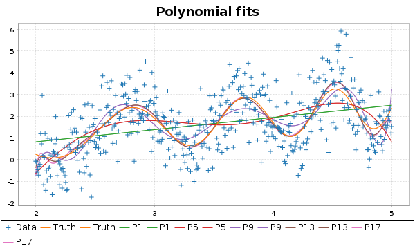
Next add some polynomial fits, using Basis.poly to generate the necessary covariate matrix.
(1 to 17 by 4).foreach(i =>
	val lm = Lm(y, Basis.poly(x, i))
	p1 += plot(x, lm.fitted, name="P"+i)
)
p1.legend = true
p1.title = "Polynomial fits"
That’s it!
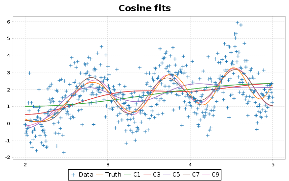
Cosine series regression
If you prefer a spectral approach to non-parametric regression, you can use cosine series instead. Lets re-use the previous data, but start a new plot.
val f2 = Figure("Cosine series")
val p2 = f2.subplot(0)
p2 += plot(x, y, '+', name="Data")
p2 += plot(x, yt, name="Truth")
Next add some cosine series fits, using Basis.cosine to generate the necessary covariate matrix.
(1 to 9 by 2).foreach(i =>
	val lm = Lm(y, Basis.cosine(x, i))
	p2 += plot(x, lm.fitted, name="C"+i)
)
p2.legend = true
p2.title = "Cosine fits"
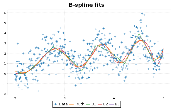
B-splines
Here, we instead use B-splines to get a flexible fit. We use 10 interior knots, and consider linear, quadratic and cubic B-spline basis functions.
val f3 = Figure("B-splines")
val p3 = f3.subplot(0)
p3 += plot(x, y, '+', name="Data")
p3 += plot(x, yt, name="Truth")
(1 to 3).foreach(i =>
	val lm = Lm(y, Basis.bs(x, i)(linspace(2.2,4.8,10).data.toIndexedSeq))
	p3 += plot(x, lm.fitted, name="B"+i)
)
p3.legend = true
p3.title = "B-spline fits"