Other topics

6.1 An example: sparse matrix computation

Many statistical computations involve matrices which contain very high proportions of zeroes: these are known as sparse matrices. Most of the computational time used by most numerical linear algebra routines is devoted to additions, subtractions and multiplications of pairs of floating point numbers: if we know, in advance, that one of the pair is a zero, we don’t actually need to perform the operation, since the answer is also known in advance. In addition, there is little point in storing all the zeroes in a sparse matrix: it is often much more efficient to store only the values of the non-zero elements, together with some encoding of their location in the matrix.

Efficient storage and simple matrix manipulations are easy to implement. Here is an example, based on simulating the model matrix for a linear model with 2 factors, and a large number of observations.

  n <- 100000 ## number of obs
  pa <- 40;pb <- 10 # numbers of factor levels
  a <- factor(sample(1:pa,n,replace=TRUE))
  b <- factor(sample(1:pb,n,replace=TRUE))
  X <- model.matrix(~a*b) # model matrix a + b + a:b
  y <- rnorm(n) # a random response
  object.size(X) # X takes lots of memory!

## 326428560 bytes

  sum(X==0)/prod(dim(X)) # proportion of zeros

## [1] 0.9906125

  library(Matrix)
  Xs <- Matrix(X) ## a sparse version of X
  ## much reduced memory footprint
  as.numeric(object.size(Xs))/as.numeric(object.size(X))

## [1] 0.03349829

  system.time(Xy <- t(X)%*%y)

##    user  system elapsed 
##   0.258   0.110   0.308

  system.time(Xsy <- t(Xs)%*%y)

##    user  system elapsed 
##   0.012   0.000   0.012

Any competent programmer could produce code for the examples given so far, but any serious application will involve solving linear systems, and this is much less straightforward. Sparse versions of some of the decompositions that we met in section 2 are needed, but naive implementations using sparse matrices flounder on the problem of infill (or fill-in). You can see the problem in the following dense calculation…

system.time({
    XX <- t(X)%*%X
    R <- chol(XX)
})

##    user  system elapsed 
##   1.837   0.114   0.728

  dim(XX)

## [1] 400 400

  sum(XX == 0)/prod(dim(XX))

## [1] 0.97935

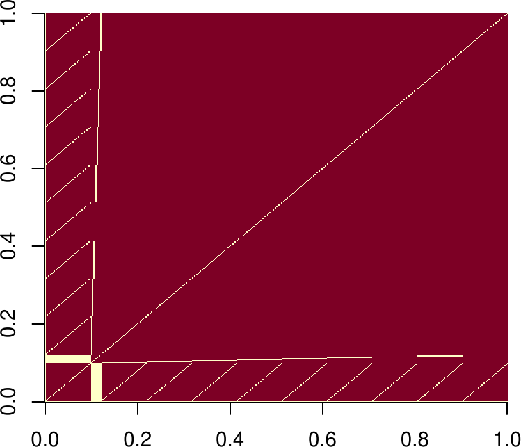
image(XX == 0)

  range(t(R)%*%R-XX)

## [1] -4.547474e-13  1.455192e-11

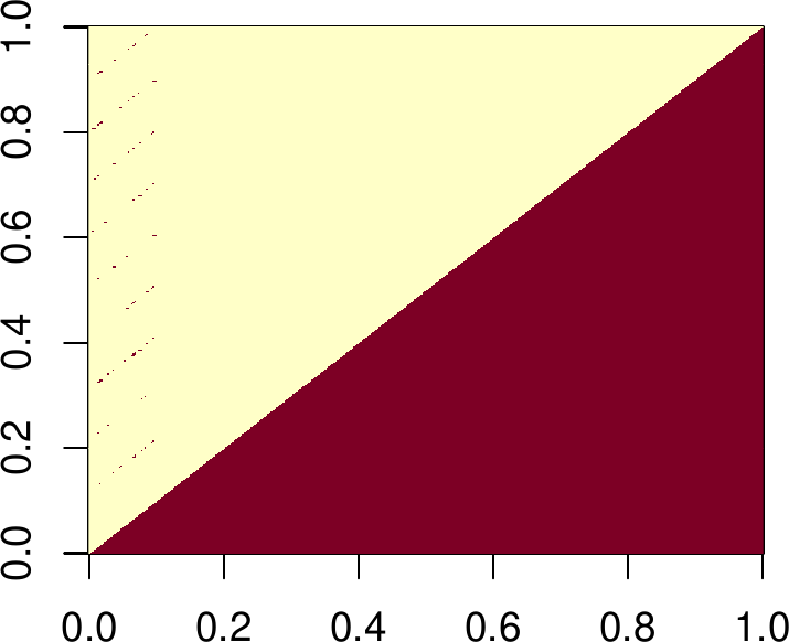
  sum(R != 0) ## the upper triangle is dense (not good)

## [1] 80113

  image(R == 0)

  R[1:5, 1:5] ## top left corner, for example

##             (Intercept)        a2        a3        a4        a5
## (Intercept)    316.2278  7.712795  7.962615  8.149190  8.051159
## a2               0.0000 48.780250 -1.258994 -1.288493 -1.272993
## a3               0.0000  0.000000 49.527888 -1.342901 -1.326747
## a4               0.0000  0.000000  0.000000 50.071220 -1.378683
## a5               0.0000  0.000000  0.000000  0.000000 49.758389

  system.time({
    XXs <- t(Xs)%*%Xs
    Rs <- chol(XXs,pivot=TRUE) ## pivot to reduce infill
  })

##    user  system elapsed 
##   0.033   0.001   0.033

  range(t(Rs)%*%Rs-XXs[Rs@pivot,Rs@pivot]) ## factorization works!

## [1] -5.684342e-14  5.684342e-14

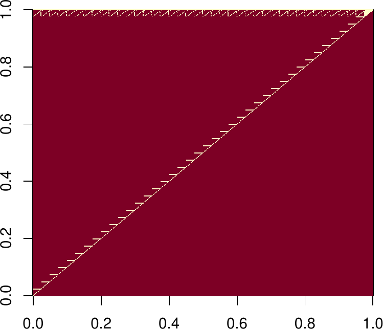
  sum(Rs!=0) ## the upper triangle is sparse (much better)

## [1] 1729

  image(as.matrix(Rs) == 0)

  Rs[1:5,1:5] ## top left corner, for example

## 5 x 5 sparse Matrix of class "dtCMatrix"
##             (Intercept)       a2       a3       a4       a5
## (Intercept)    14.89966  .        .        .        .      
## a2              .       15.93738  .        .        .      
## a3              .        .       15.36229  .        .      
## a4              .        .        .       16.18641  .      
## a5              .        .        .        .       15.96872

Note that while the sparse Cholesky routines in the Matrix package are state-of-the-art, the QR routines are not, and carry heavy memory overheads associated with computation of ${\bf Q}$. You’ll probably need to look for sparse multi-frontal QR routines if you need sparse QR.

6.2 Hashing: another example

Suppose that you want to store data, which is to be accessed using arbitrary keys. For example, you want to store data on a large number of people, using their names (as a text string) as the key for finding the record in memory. i.e., data about someone is read in from somewhere, and is stored at a location in computer memory, depending on what their name string is. Later you want to retrieve this information using their name string. How can you actually do this?

You could store some sort of directory of names, which would be searched through to find the location of the data. But such a search is always going to take some time, which will increase with the number of people’s data that is stored. Can we do better? With hashing the answer is yes. The pivotal idea is to create a function which will turn an arbitrary key into an index which is either unique or shared with only a few other keys, and has a modest predefined range. This index gives a location in a (hash) table which in turn stores the location of the actual data (plus some information for resolving ‘clashes’). So given a key, we use the (hash) function to get its index, and its index to look up the data location, with no, or very little searching. The main problem is how to create a hash function.

An elegant general strategy is to use the ideas of pseudorandom number generation to turn keys into random integers. For example, if the key were some 64bit quantity, we could use it to seed the Xorshift random number generator given earlier, and run this forward for a few steps. More generally we would need an approach that successively incorporated all the bits in a key into the ‘random number’ generation process (see e.g. section 7.6 of Press et al., 2007, for example code). So, the hash function should return numbers that appear random, which will mean that they tend to be nicely spread out, irrespective of what the keys are like. Of course, despite this, the function always returns the same number for a given key.

It remains to turn the number returned by the hash function, $h$, into an index, $i_ h$ , somewhere between 0 and the length, $n_ h$, of the hash table minus 1. $i_ h = h~ {\rm mod}~ n_ h$ is the usual approach. At position $i_ h$ in the hash table we might store the small number of actual keys (or possibly just their $h$ values) sharing the $i_ h$ value, and the actual location in memory of the corresponding data.

The really neat thing here is that the randomness of the $h$’s means that whatever the keys look like, you usually end up with a fairly uniform distribution of $i_ h$’s, and only a small number of keys sharing each slot in the hash table. It is this that makes data retrieval so efficient, relative to searching a directory of keys.

Note that R environments are themselves methods for associating values with lookup keys, and in fact, R environments can use hash tables.

ht <- new.env(hash=TRUE)
ht[["foo"]] = "bar"
ht[["baz"]] = 1:10
ht[["foo"]]

## [1] "bar"

ht$baz

##  [1]  1  2  3  4  5  6  7  8  9 10

If that doesn’t sound like it has any application in statistics, consider the construction of triangulations in spatial statistics (a triangulation being a way of joining a set of points up with triangles, in such a way that the whole complex hull of the points is covered in triangles). Efficient construction of triangulations is tricky, and several efficient algorithms work by incrementally adding triangles. You usually know at least one neighbour of each triangle at its creation, but you actually need to know all its neighbours in the existing set. The task of finding those neighbours would be prohibitive if you had to search each existing triangle for edges shared with the new triangle. Instead one can maintain a hash table for unpaired triangle edges, where the hash key is based on the end co-ordinates of each edge. This allows any newly created edge to be paired with any existing edge in little more than the length of time it takes to create the hash key.

6.3 Further reading

1. 1.

   For a good introduction to the sparse methods underlying Martin Maechler and Douglas Bates’ R package Matrix, see Davis, T. A. (2006) Direct Methods for Sparse Linear Systems, SIAM.

2. 2.

   Tim Davis’s home page is worth a look for more recent sparse matrix developments
   http://faculty.cse.tamu.edu/davis/research.html.

3. 3.

   If you think hashing is clever, take a look at the rest of Cormen, T., C.E. Leiserson, R.L. Rivest and C. Stein (2001) Introduction to Algorithms (2nd ed.) MIT.

4. 4.

   Once again, Press, W.H., S.A. Teukolsky, W.T. Vetterling and B.P Flannery (2007) Numerical Recipes (3rd ed.) provides a readable introduction to a much wider range of topics in scientific computing than has been covered here.