MATH4341: Spatio-temporal statistics
Term 2: Spatial modelling and analysis
Computer Lab 7: CAR priors and sparse matrices
Load up RStudio via your favourite method. If you can’t use RStudio for some reason, most of what we do in these labs can probably be done using WebR, but the instructions will assume RStudio. You will also want to have the web version of the lecture notes to refer to.
Question 1
If you haven’t already done so, reproduce all of the plots and computations from Chapter 15 of the lecture notes by copying and pasting each code block in turn. Make sure you understand what each block is doing and that you can reproduce all of the plots.
Question 2
Today we will be primarily concerned with data relating to districts within New York, spData::nydata. The actual data of interest relates to incidence of leukemia, but we will be mainly concerned with the development of CAR priors over New York tracts (districts). First, load some libraries.
A basic data frame containing the data is exported by default.
dim(nydata)[1] 281 12head(nydata) AREANAME AREAKEY X Y POP8 TRACTCAS PROPCAS
1 Binghamton city 36007000100 4.069397 -67.3533 3540 3.08 0.000870
2 Binghamton city 36007000200 4.639371 -66.8619 3560 4.08 0.001146
3 Binghamton city 36007000300 5.709063 -66.9775 3739 1.09 0.000292
4 Binghamton city 36007000400 7.613831 -65.9958 2784 1.07 0.000384
5 Binghamton city 36007000500 7.315968 -67.3183 2571 3.06 0.001190
6 Binghamton city 36007000600 8.558753 -66.9344 2729 1.06 0.000388
PCTOWNHOME PCTAGE65P Z AVGIDIST PEXPOSURE
1 0.3277311 0.1466102 0.14197 0.2373852 3.167099
2 0.4268293 0.2351124 0.35555 0.2087413 3.038511
3 0.3377396 0.1380048 -0.58165 0.1708548 2.838229
4 0.4616048 0.1188937 -0.29634 0.1406045 2.643366
5 0.1924370 0.1415791 0.45689 0.1577753 2.758587
6 0.3651786 0.1410773 -0.28123 0.1726033 2.848411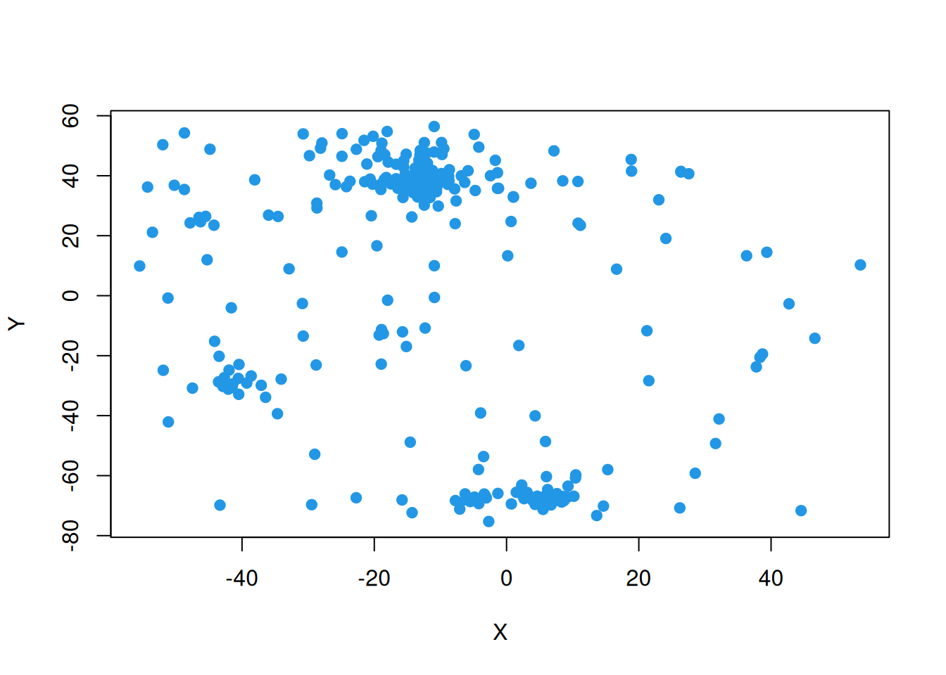
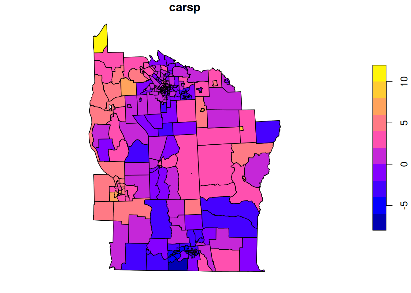
The main variable of interest is Z, which we can look at simply as follows.
hist(nydata$Z, col=4)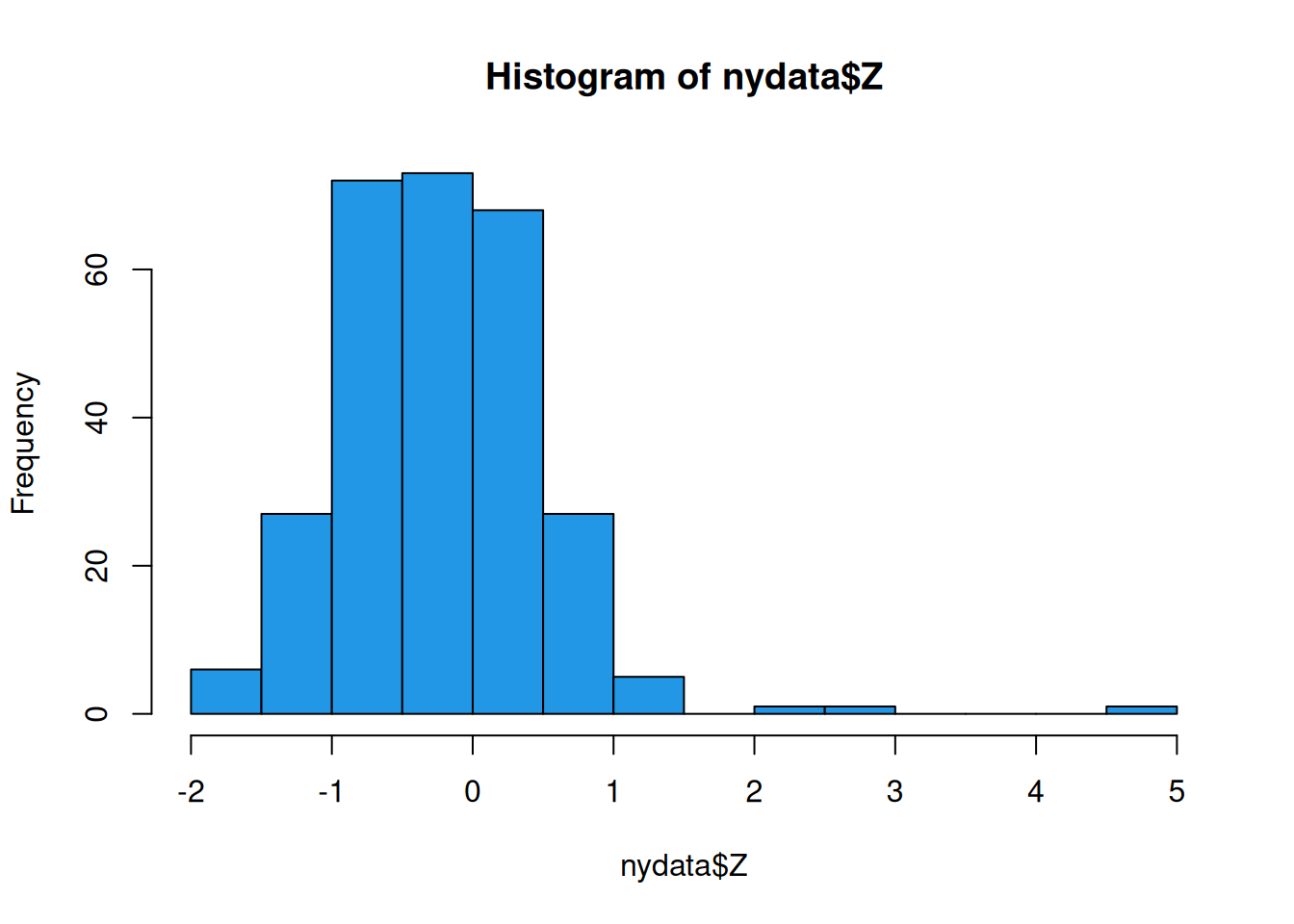
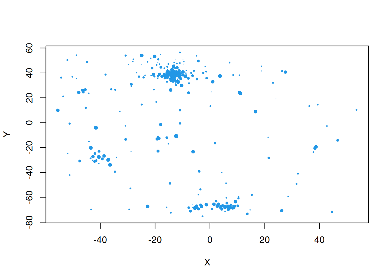
Since Z is a z-score, we can map it to \((0,1)\) by applying pnorm and using that as a point size to plot.
For further exploration, it would be helpful to have the full geometry of the regions of interest. We can load this data as follows.
nyd = st_read(system.file("shapes/NY8_bna_utm18.gpkg",
                          package="spData"))
Now we can plot the variable of interest as a choropleth map.
plot(nyd[,"Z"])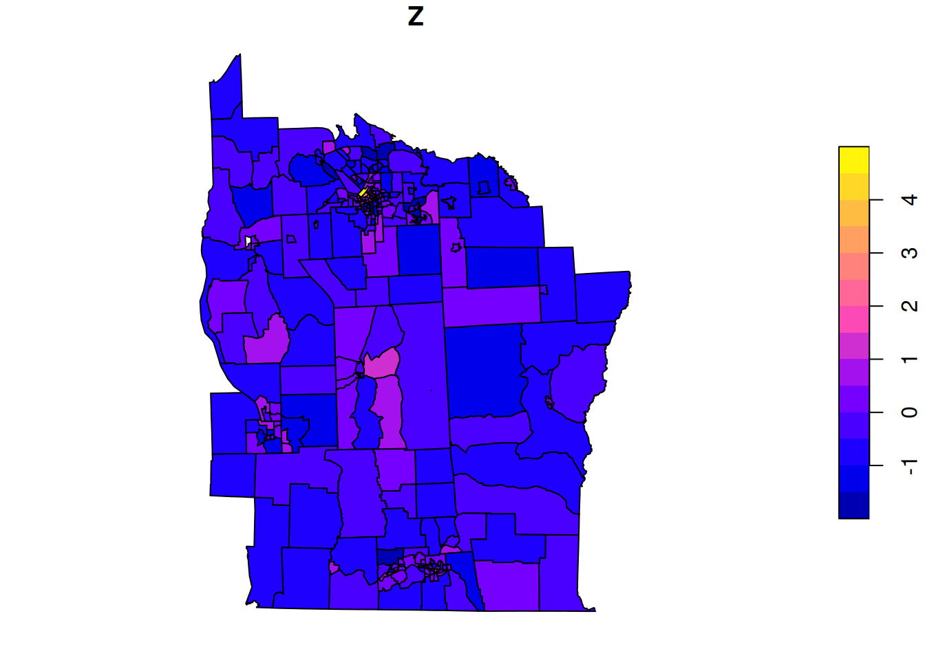
2.1
In this practical lab we are less interested in the data, and more interested in the specification of a CAR prior over NY tracts. For this we need a neighbourhood structure. Although there are other things we could do, it is natural to consider neighbours as tracts with common boundaries. We can use the function spdep::poly2nb for this.
nyd_nb = spdep::poly2nb(nyd)
nyd_nb
Neighbour list object:
Number of regions: 281
Number of nonzero links: 1632
Percentage nonzero weights: 2.066843
Average number of links: 5.807829 The result is a list with one element per tract. Each element is a vector of neighbours of the relevant tract.
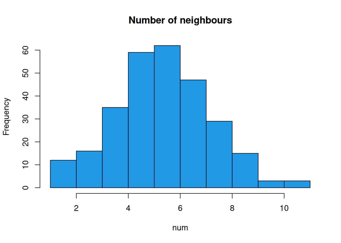
So, there are 281 tracts. The first tract has 8 neighbours, and the second has 6. We can plot the graph of the neighbourhood structure as follows.
plot(st_geometry(nyd), border="lightgrey")
plot(nyd_nb, sf::st_geometry(nyd), pch=19, cex=0.7,
add=TRUE, col="blue")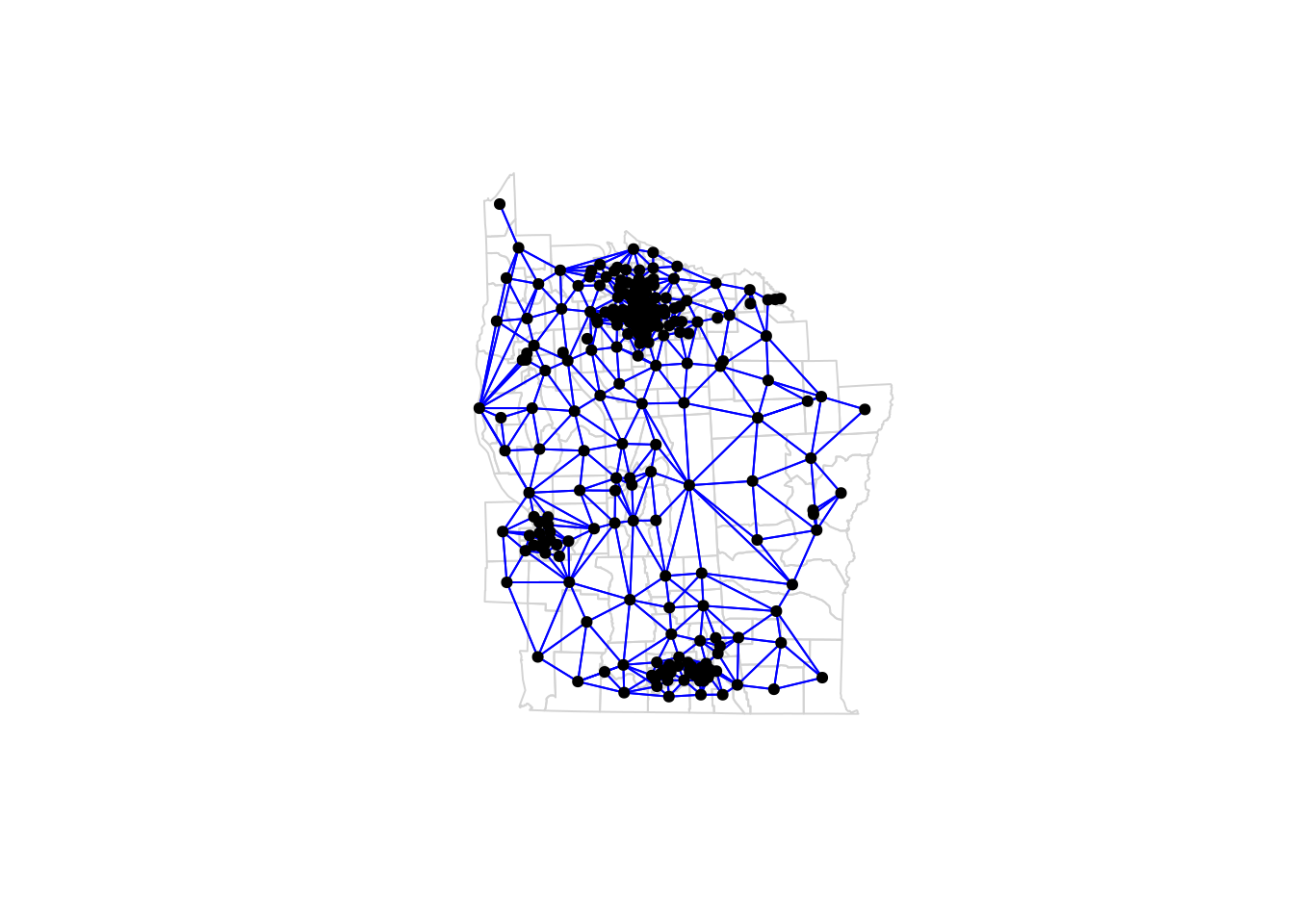
So, now that we have a graph, we can think about defining a CAR prior on it. The function spdep::nb2mat will create a row-normalised adjacency matrix.
adjW = spdep::nb2mat(nyd_nb)
isSymmetric(adjW)[1] FALSEadjW[1:5,1:5] 1 2 3 4 5
1 0.0000000 0.1250000 0.0000000 0.0000000 0.0000000
2 0.1666667 0.0000000 0.1666667 0.0000000 0.0000000
3 0.0000000 0.1666667 0.0000000 0.1666667 0.1666667
4 0.0000000 0.0000000 0.2500000 0.0000000 0.2500000
5 0.0000000 0.0000000 0.1666667 0.1666667 0.0000000 Min. 1st Qu. Median Mean 3rd Qu. Max.
1 1 1 1 1 1 Task A
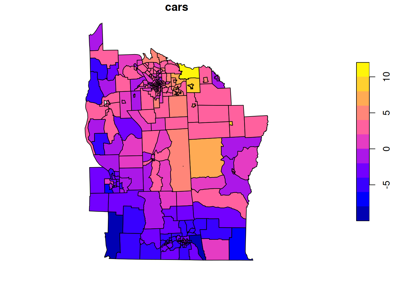
Use this adjacency matrix to simulate from an equally weighted CAR prior with \(\kappa=1\) and \(\rho=0.999\). Plot the sample as a choropleth map.
2.2
It is very often convenient and desirable to use a CAR prior with equal weight on each neighbour, but it is by no means necessary. For a prior that is not equally weighted, it is simplest to start from a set of neighbour weights that is symmetric. These weights can be arranged in a sparse symmetric matrix, \(\mathsf{W}\), with non-zero elements corresponding to neighbours. The distance between the centroids of the regions of interest is an example of a symmetric weight; the distance from region \(i\) to region \(j\) is the same as the distance from region \(j\) to region \(i\). Typically we would want more weight for regions that are near than regions that are distant, so a function such as a reciprocal could be applied to distance to obtain a suitable symmetric weight function. Alternatively, the absolute length of a common border could be used as a symmetric weight for a nearest neighbour graph structure. Given such a symmetric weight function, a consistent CAR model can be specified via the local characteristics \[ (Z_i|\mathbf{Z}_{-i}=\mathbf{z}_{-i}) \sim \mathcal{N}\left( \rho\sum_j \frac{ w_{ij}}{\sum_k w_{ik}} z_j , \frac{\kappa}{\sum_k w_{ik}} \right). \] So, although the weight matrix is symmetric, the weights applied to adjacent regions are not, since they are row-normalised. eg. if the weight is absolute length of a common border, the weights at region \(i\) applied to neighbours \(j\) will be the proportion of the total length of the border of region \(i\) accounted for by region \(j\). This is obviously not symmetric with region \(j\), but makes intuitive sense.
We know that for consistency, and in particular, the symmetry of the precision matrix, we must have \(a_{ij}/\kappa_i = a_{ji}/\kappa_j\). But here we have \[ \frac{a_{ij}}{\kappa_i} = \frac{\displaystyle \rho\frac{w_{ij}}{\sum_k w_{ik}}}{\displaystyle \frac{\kappa}{\sum_k w_{ik}}} = \rho\frac{w_{ij}}{\kappa}, \] and so provided that \(\mathsf{W}\) is symmetric (and \(\rho\in(0,1)\), for diagonal dominance), this specification will be consistent.
We will illustrate with weights corresponding to the reciprocal of the distance between centroids of the neighbouring regions.
dlist = spdep::nbdists(nyd_nb, st_coordinates(st_centroid(nyd)))
wlist = lapply(dlist, function(x) 1/x) # weights list
rowsums = sapply(wlist, sum)
nyd_w = spdep::nb2listw(nyd_nb, glist=wlist)
nyd_wCharacteristics of weights list object:
Neighbour list object:
Number of regions: 281
Number of nonzero links: 1632
Percentage nonzero weights: 2.066843
Average number of links: 5.807829
Weights style: W
Weights constants summary:
n nn S0 S1 S2
W 281 78961 281 126.83 1147.906The weights list is a list of vectors of row-normalised weights. We can use spdep::listw2mat to turn this into a sparse weight matrix.
[1] 281 281adjWD[1:5,1:5] 1 2 3 4 5
1 0.0000000 0.1975860 0.0000000 0.0000000 0.0000000
2 0.2673439 0.0000000 0.2026457 0.0000000 0.0000000
3 0.0000000 0.2290087 0.0000000 0.1473584 0.1579192
4 0.0000000 0.0000000 0.1759369 0.0000000 0.2763971
5 0.0000000 0.0000000 0.1176839 0.1725176 0.0000000 Min. 1st Qu. Median Mean 3rd Qu. Max.
1 1 1 1 1 1 Task B
Use this weight matrix to sample from a CAR prior (with same \(\kappa\), \(\rho\) as before), and plot it.
Question 3
3.1
We have talked a lot about the sparsity of the precision matrix in CAR models, and in graphical models and Markov random fields more generally. We have also noted that the sparsity of matrices can be exploited to reduce storage and computation. But so far we have been using regular dense matrix algorithms for all of our examples. We can fix this now.
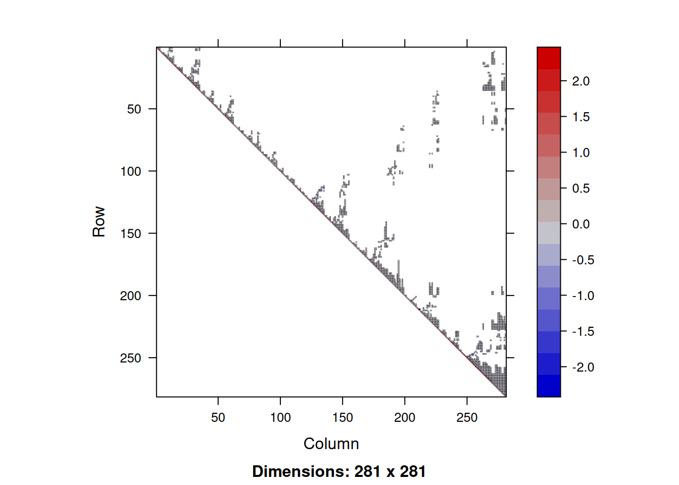
Let’s start by looking at the sparsity of the distance-weighted adjacency matrix we have just been considering.
image(adjWD)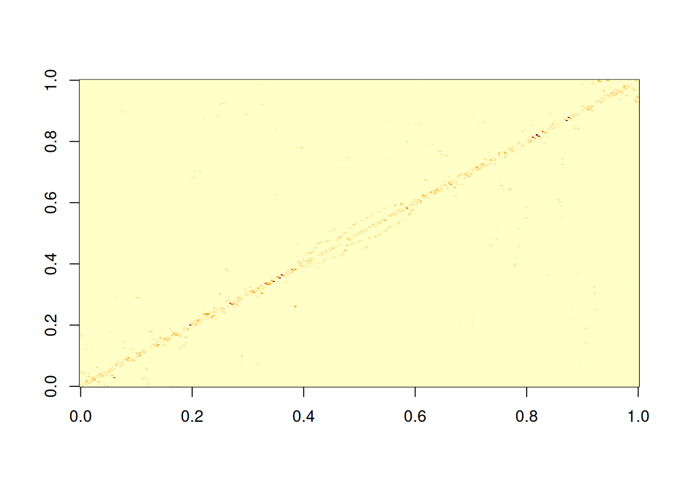
It would be better to rearrange rows and columns to plot in a more intuitive way.
We see that there are lot of non-zero elements close to the main diagonal, but a bunch of other non-zero values scattered elsewhere. We can quantify the sparsity by looking at the fraction of elements that are zero.
So around 98% of the elements of this matrix are zero. This means that we are storing lots of zeros in memory, and computations involving this matrix will involve lots of multiplications by zero that could be avoided. Any reasonable size matrix with a large fraction (say, more than 90%) of zeros can be considered to be sparse, and would be better treated using specialist sparse matrix libraries. There are several R packages for dealing with sparse matrices. We will use the Matrix package, which you should already have installed, since it is a dependency of spatialreg, but can be installed from CRAN in the usual way.
The spatialreg library includes code for converting neighbour weight lists into sparse matrices.
[1] "dgCMatrix"
attr(,"package")
[1] "Matrix"adjS[1:5, 1:5]5 x 5 sparse Matrix of class "dgCMatrix"
1 2 3 4 5
1 . 0.1975860 . . .
2 0.2673439 . 0.2026457 . .
3 . 0.2290087 . 0.1473584 0.1579192
4 . . 0.1759369 . 0.2763971
5 . . 0.1176839 0.1725176 . adjWD[1:5, 1:5] 1 2 3 4 5
1 0.0000000 0.1975860 0.0000000 0.0000000 0.0000000
2 0.2673439 0.0000000 0.2026457 0.0000000 0.0000000
3 0.0000000 0.2290087 0.0000000 0.1473584 0.1579192
4 0.0000000 0.0000000 0.1759369 0.0000000 0.2763971
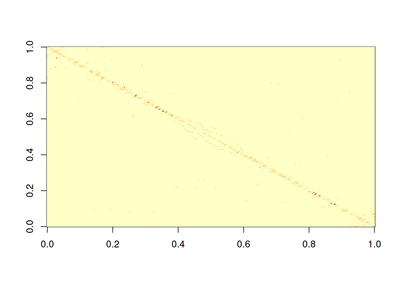
5 0.0000000 0.0000000 0.1176839 0.1725176 0.0000000So adjS is a sparse matrix equivalent to adjWD. It contains the same elements, but importantly, the sparse matrix version only stores the non-zero matrix elements, which means it takes up much less RAM.
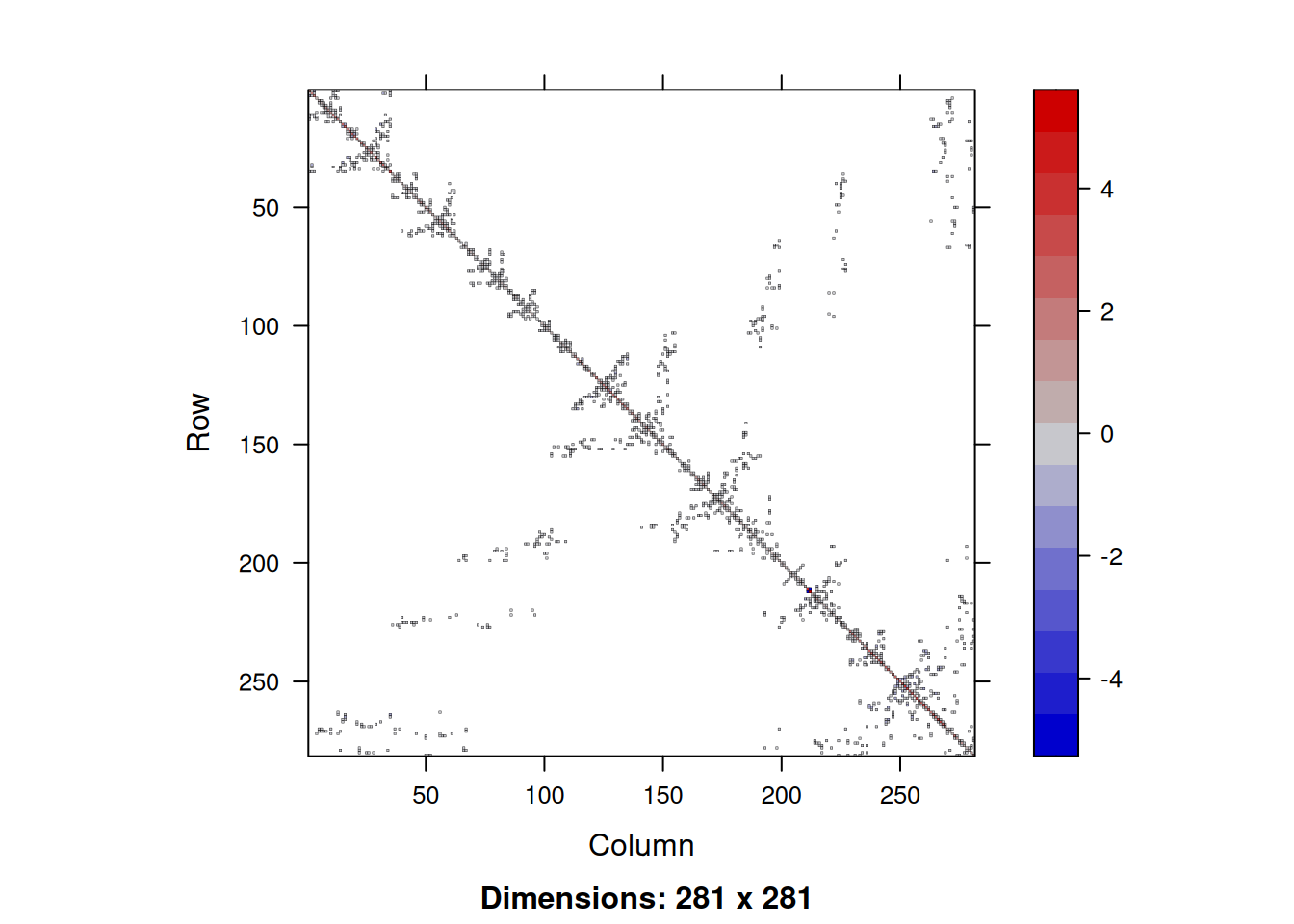
object.size(adjS)58272 bytesobject.size(adjWD)668144 bytesas.numeric(object.size(adjS)/object.size(adjWD))[1] 0.08721473So we see that even with this rather small and simple example, the size of the sparse matrix is only around 9% of the size of the corresponding dense version. This is more than the 2% you might have expected, but that is because for sparse matrices we need to store the location of the non-zero elements, as well as their values. We can image the sparsity structure of sparse matrices using the image function.
image(adjS)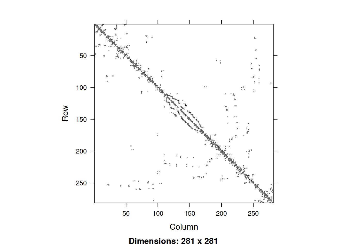
Note that the image is automatically oriented in the intuitive way. We can use the usual operations on sparse matrices, and sparse diagonal matrices can be constructed with the Diagonal function. So we can create a sparse precision matrix for our CAR prior as follows.
kappa = 1
rho = 0.999
Kv = mean(rowsums) * kappa / rowsums
As = adjS * rho
Qs = (Diagonal(n) - As)/Kv
Qs[1:5, 1:5]
5 x 5 sparse Matrix of class "dgCMatrix"
1 2 3 4 5
1 2.1936389 -0.4329989 . . .
2 -0.4329989 1.6212539 -0.3282116 . .
3 . -0.3282116 1.4346186 -0.2111917 -0.2263273
4 . . -0.2111917 1.2015846 -0.3317824
5 . . -0.2263273 -0.3317824 1.9251055image(Qs)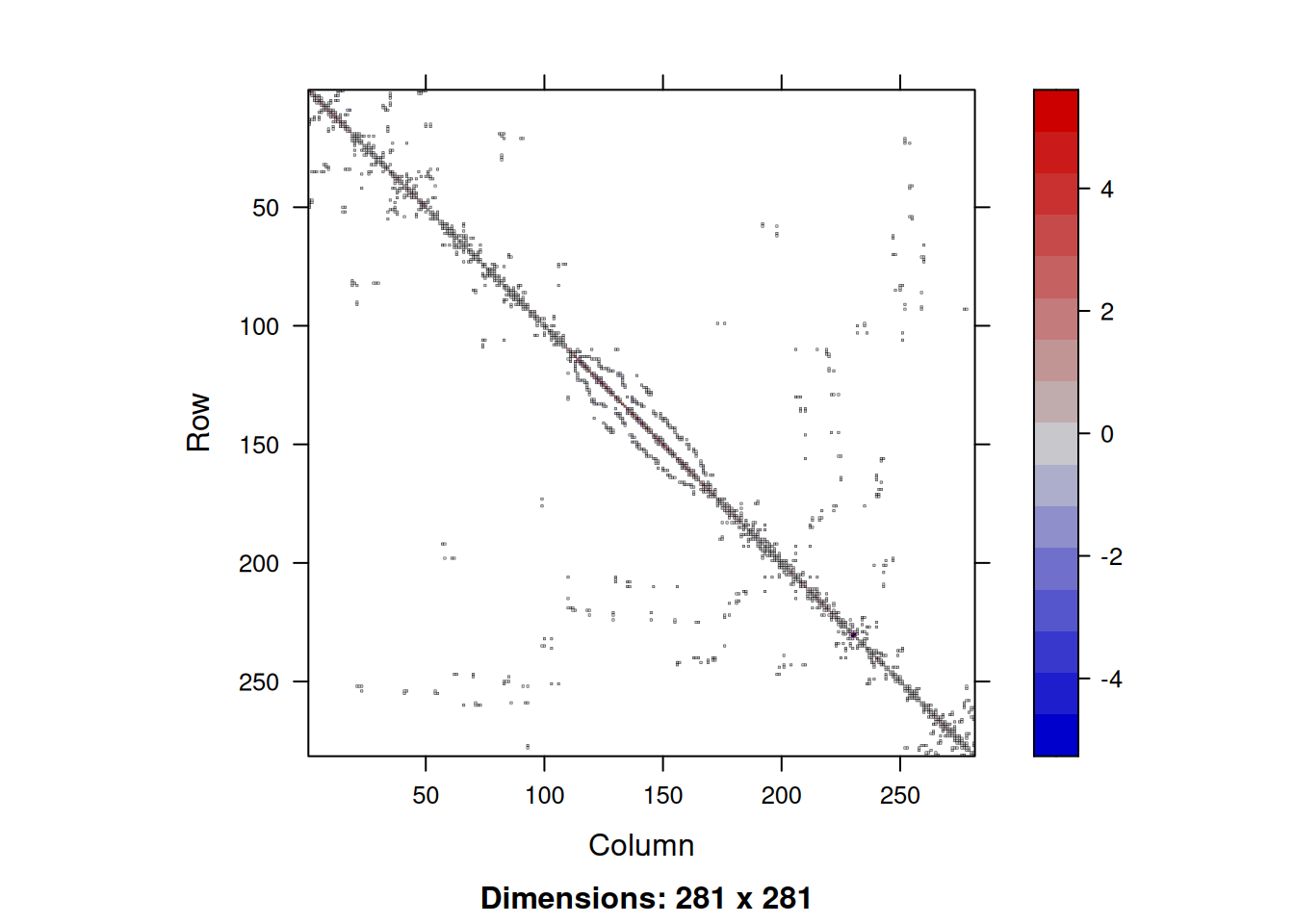
If we want to generate a sample from this CAR prior, we know that we can do this by forming the Cholesky decomposition of the precision matrix, and then back-solving this against a vector of standard normals. We can use the chol function on a sparse matrix to get a sparse (upper) Cholesky triangle.
The result is an upper-triangular sparse matrix, and the matrix object contains attributes which indicate this. If we look at the Cholesky factor,
image(Lts)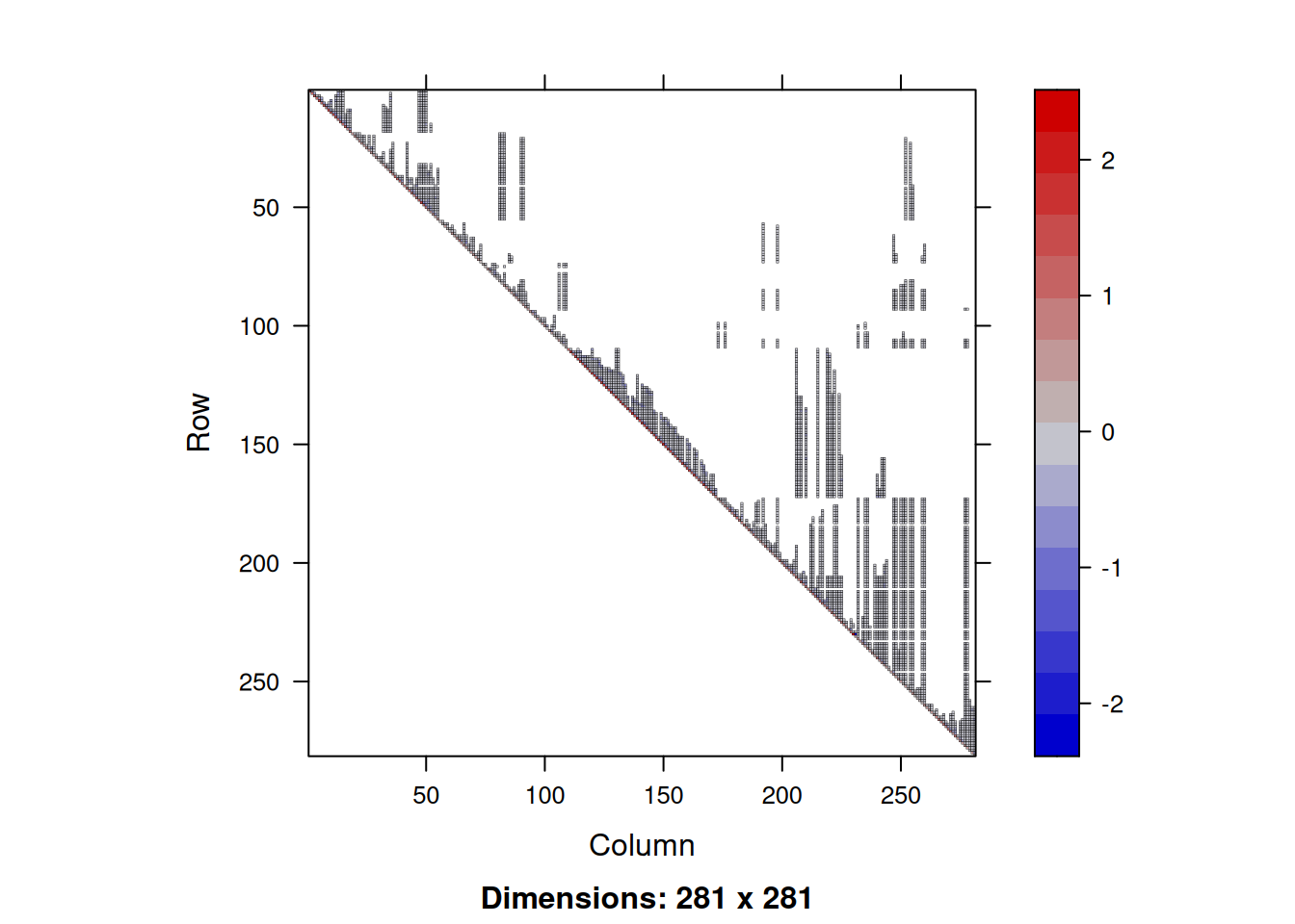
we see that it is sparse, but less sparse than the precision matrix. The additional non-zero elements are known as fill-in. It is possible to reduce the fill-in by carefully permuting the rows and columns of the precision matrix prior to factorisation, but we will look at that later. We can solve against a vector of standard normals using Matrix::solve. Note that this function will know to back-solve this system since the sparse matrix Lts is labelled as upper triangular.
This gives us a way to sample from CAR models without ever building an \(n\times n\) dense matrix. Although for this small problem using dense matrix methods worked fine, for models with thousands of nodes, sparse matrix methods are transformative.
3.2
So, we now know how to use sparse matrix methods to sample from GGMs. But we noted that the Cholesky factor of the precision matrix was significantly less sparse than the precision matrix. Let’s quantify this.
So here the loss of sparsity is tolerable, but it is very often the case that the loss of sparsity is catastrophic. So let’s see if we can do better. We know that the Cholesky factor of \(\mathsf{Q}\) is (typically) a lower triangular matrix, \(\mathsf{L}\), such that \(\mathsf{Q}=\mathsf{L}\mathsf{L}^\top\). We know that R has a quirk of returning the upper triangle, \(\mathsf{L}^\top\), but that isn’t a big deal.
Qs[1:5, 1:5]5 x 5 sparse Matrix of class "dgCMatrix"
1 2 3 4 5
1 2.1936389 -0.4329989 . . .
2 -0.4329989 1.6212539 -0.3282116 . .
3 . -0.3282116 1.4346186 -0.2111917 -0.2263273
4 . . -0.2111917 1.2015846 -0.3317824
5 . . -0.2263273 -0.3317824 1.92510555 x 5 sparse Matrix of class "dgCMatrix"
1 2 3 4 5
1 2.1936389 -0.4329989 . . .
2 -0.4329989 1.6212539 -0.3282116 . .
3 . -0.3282116 1.4346186 -0.2111917 -0.2263273
4 . . -0.2111917 1.2015846 -0.3317824
5 . . -0.2263273 -0.3317824 1.9251055It turns out that the fill-in of a Cholesky decomposition can be greatly reduced by first permuting the rows and columns of \(\mathsf{Q}\) in an appropriate way. There are heuristic algorithms for doing this that work very well in practice. So, rather than decomposing \(\mathsf{Q}\), we decompose \(\mathsf{P}\mathsf{Q}\mathsf{P}^\top\), where \(\mathsf{P}\) is a permutation matrix. So then \[
\mathsf{P}\mathsf{Q}\mathsf{P}^\top = \mathsf{L}\mathsf{L}^\top,
\] or equivalently, \[
\mathsf{Q} = \mathsf{P}^\top\mathsf{L}\mathsf{L}^\top\mathsf{P}.
\] The Cholesky function can perform this decomposition for us, though we must use the expand2 function to turn the internal representation into a list of sparse factors.
[1] "P1." "L" "L." "P1" The factor L. is \(\mathsf{L}^\top\).
So we see that this has significantly more sparsity than the unpermuted Cholesky factor. If we look at the permuted \(\mathsf{Q}\) matrix, we see that the off-diagonal elements are less randomly scattered.
To sample from our CAR model, we can solve our Cholesky factor against a vector of standard normals, but we must then remember to undo the permutation to get back to our original variable ordering.
This works because \[\begin{align*} \text{Var}(\mathbf{X}) &= \text{Var}(\mathsf{P}^\top[\mathsf{L}^{\top-1}\mathbf{Z}]) \\ &= \text{Var}([\mathsf{P}^\top\mathsf{L}^{\top-1}]\mathbf{Z}) \\ &= \mathsf{P}^\top\mathsf{L}^{\top-1}\text{Var}(\mathbf{Z})\mathsf{L}^{-1}\mathsf{P} \\ &= \mathsf{P}^\top\mathsf{L}^{\top-1}\mathsf{L}^{-1}\mathsf{P} \\ &= \mathsf{P}^\top(\mathsf{L}\mathsf{L}^{\top})^{-1}\mathsf{P} \\ &= \mathsf{P}^\top(\mathsf{P}\mathsf{Q}\mathsf{P}^\top)^{-1}\mathsf{P} \\ &=\mathsf{Q}^{-1}, \end{align*}\] as required.
Although this problem is rather small and unproblematic, in general, using fill-reducing permutations can greatly improve the performance of sparse-matrix algorithms. Together, the use of fill-reducing permutations and sparse matrix algorithms allow the analysis of MRFs with tens of thousands of nodes with relative ease. You just sometimes need to think carefully about how to unscramble things correctly at the end.