We now turn attention to the problem of building joint probability distributions over a lattice of sites. In particular, we would like to extend the concept of an auto-regressive model from time series to spatial data. Unfortunately, due to the lack of natural ordering on spatial locations, this is not completely straightforward. In particular, there is more than one way to do it, and they are not equivalent. Regardless, we would somehow like to make some kind of specification regarding the distribution at individual sites, and then use these to build a full joint distribution. Specifying conditional distributions is one natural way to do this, so we begin by thinking about how and when conditional distributions specify a joint distribution.
15.1.1 Compatible distributions
Given a joint distribution for a pair of random quantities \(X\) and \(Y\), we know that we can factor it into a product of a marginal and a conditional two different ways, \[
f_{X,Y}(x, y) = f_X(x)f_{Y|X}(y|x) = f_Y(y)f_{X|Y}(x|y),
\] and that both of these factorisations can be useful. But now suppose that we are only given the two conditional distributions, \(f_{X|Y}(x|y)\) and \(f_{Y|X}(y|x)\). Do these two conditional distributions uniquely determine the joint distribution, and if so, can we deduce it? Furthermore, given two arbitrary conditional distributions, can we tell if they are consistent with any joint distribution at all? In general, not all possible pairs of conditional distributions do determine a well-defined joint distribution. When they do, we say that the conditionals are compatible.
Proposition (Compatible distributions)
Conditional densities \(f_{X|Y}(x|y)\) and \(f_{Y|X}(y|x)\) are compatible if they have the same support and there exist functions \(u(x)\) and \(v(y)\) such that \[
\frac{f_{X|Y}(x|y)}{f_{Y|X}(y|x)} = u(x)v(y), \quad \text{where} \quad \int_\mathbb{R} u(x)\,\mathrm{d}x < \infty.
\] That is, the ratio of densities factorises into separate functions of \(x\) and \(y\), and the function of \(x\) is integrable.
Proof. (sketch) If \(f_{X,Y}(x, y)\) exists with marginals \(f_X(x)\) and \(f_Y(y)\), then \(f_X(x)f_{Y|X}(y|x) = f_Y(y)f_{X|Y}(x|y)\) implies \[
\frac{f_{X|Y}(x|y)}{f_{Y|X}(y|x)} = \frac{f_X(x)}{f_Y(y)} = u(x)v(y),
\] where \(u(x)=f_X(x)\) and \(v(y) = 1/f(y)\). Clearly \(u\) and \(v\) are determined only up to a multiplicative constant, but since \(f_X(x)\) integrates to one, \(u(x)\) must be integrable.
Note that normalising \(u(x)\) will give \(f_X(x)\), and together with \(f_{Y|X}(y|x)\), this gives the joint distribution.
So this proposition gives us a way of checking compatibility, and in the case of compatibility, gives us a way to compute the associated joint distribution. We will later see an easier way to construct the joint in situations where we know the conditionals are compatible.
15.1.1.1 Example: AR(1)
Let \(X\) and \(Y\) be two consecutive values of an AR(1) model (eg. \(X_t\) and \(X_{t+1}\)). We know that the conditional density for \(Y|X\) is \[
f_{Y|X}(y|x) = \mathcal{N}(y;\alpha x, \sigma^2),
\] but in the stationary case (\(|\alpha|<1\)) we know that the process is time-reversible, so we must also have \[
f_{X|Y}(x|y) = \mathcal{N}(x;\alpha y, \sigma^2).
\] In this case we know that the conditionals are compatible, and determine the joint distribution of a pair of values from a stationary AR(1) model, but let’s check, anyway. We form the ratio of conditional densities and simplify to find \[
\frac{f_{X|Y}(x|y)}{f_{Y|X}(y|x)} = u(x)v(y),
\] where \[
u(x) = \exp\left\{-\frac{1-\alpha^2}{2\sigma^2}x^2\right\}, \quad \text{and} \quad v(y) = \exp\left\{\frac{1-\alpha^2}{2\sigma^2}y^2\right\}.
\] So the ratio does indeed factorise into separate functions of \(x\) and \(y\), and further, \(u(x)\) is integrable, since it normalises to \[
f_X(x) = \mathcal{N}\left(x;0,\frac{\sigma^2}{1-\alpha^2}\right),
\] the stationary distribution of the AR(1), as we would expect.
Before moving on it is worth briefly considering the case \(\alpha=1\). This corresponds to the (non-stationary) random walk model. Here the ratio of conditionals simplifies to 1. We can write this in the form \(u(x)=1\), \(v(y)=1\), but \(u(x)\) is not integrable in this case. So the conditionals for the random walk model are not compatible, and do not correspond to a (proper) joint distribution. However, it turns out that they do in fact correspond to an improper joint distribution, analogous to the intrinsically stationary distributions we considered in continuous space. Such improper random walk priors are actually used quite often in spatial statistics, but the technical details will not concern us.
15.1.2 Conditional versus simultaneous specification
We have just seen in the above example that the conditional specifications \[\begin{align*}
f_{X|Y}(x|y) &= \mathcal{N}(x;\alpha y, \sigma^2),\\
f_{Y|X}(y|x) &= \mathcal{N}(y;\alpha x, \sigma^2),
\end{align*}\] correspond to a pair of consecutive values from a stationary AR(1) model with stationary variance \(\sigma^2/(1-\alpha^2)\). In the time series part of the course we regularly moved back-and-forth between conditional specifications like this and equational representations. We might therefore be tempted to write down an equational form of this conditionally specified model as the simultaneous system \[\begin{align*}
X &= \alpha Y + \varepsilon_1 \\
Y &= \alpha X + \varepsilon_2,
\end{align*}\] where \(\varepsilon_1\) and \(\varepsilon_2\) are independent mean zero Gaussians with variance \(\sigma^2\). We will see shortly that this is a perfectly reasonable model, and does correspond to a perfectly reasonable joint distribution over \(X\) and \(Y\). However, it is very important to understand that this is not the same as the conditional model above, and in particular, does not correspond to a pair of values from an AR(1) process. Great care should therefore be used in the interpretation of simultaneously specified models.
We can solve for the joint distribution by writing the model in matrix form as \[
\begin{pmatrix}1&-\alpha\\-\alpha&1\end{pmatrix}\binom{X}{Y} = \binom{\varepsilon_1}{\varepsilon_2},
\] from which we deduce \[
\binom{X}{Y} = \begin{pmatrix}1&-\alpha\\-\alpha&1\end{pmatrix}^{-1}\binom{\varepsilon_1}{\varepsilon_2}
= \frac{1}{1-\alpha^2}\begin{pmatrix}1&\alpha\\\alpha&1\end{pmatrix}\binom{\varepsilon_1}{\varepsilon_2}.
\] It is now clear that \(X\) and \(Y\) are jointly Gaussian with mean zero and variance matrix \[
\frac{\sigma^2}{(1-\alpha^2)^2}\begin{pmatrix}1&\alpha\\\alpha&1\end{pmatrix}^2 = \frac{\sigma^2}{(1-\alpha^2)^2}\begin{pmatrix}1+\alpha^2&2\alpha\\2\alpha&1+\alpha^2\end{pmatrix}.
\] In particular, note that the marginal variance of \(X\) (and \(Y\)) is \[
\frac{1+\alpha^2}{(1-\alpha^2)^2}\sigma^2,
\] which is not the stationary variance of an AR(1) model. There are many ways to understand why the two different approaches to specification are different (they just are!), but it may be helpful to note that in the simultaneously specified model, both errors are correlated with both\(X\) and \(Y\), which is not the case for the conditional specification. Essentially, in the simultaneous specification, the full error distribution is assumed (and the errors are assumed to be independent of each other), and this then determines the distribution of the variables (here, \(X\) and \(Y\)). OTOH, in the conditional specification, the marginal distribution of the errors is assumed, and each error is assumed to be independent of the other variables, but the distribution this induces for the variables in turn determines the joint distribution of the errors, which typically will not be independent of each other.
15.2 Simultaneous auto-regressive (SAR) models
Consider the development of a joint model for \(n\) spatial locations. Inspired by the equational form of an auto-regressive time series model, we could model each location as a linear combination of the others plus some residual error. \[
Z_i = \sum_{j\not= i} b_{ij} Z_j + \varepsilon_i, \quad \varepsilon_i\sim\mathcal{N}(0,\sigma_i^2),\quad i=1,2,\ldots,n.
\] This kind of simultaneous specification is very closely related to the simultaneous equations models that are widely used in econometrics. Just as an auto-regressive time series model does not depend on all previous observations, we would expect that most \(b_{ij}\) will be 0. The coefficient \(b_{ij}\) will be non-zero only when \(Z_j\) has a “direct” influence on \(Z_i\). We can write the model in matrix form as \[
\mathbf{Z} = \mathsf{B}\mathbf{Z} + \pmb{\varepsilon},\quad \pmb{\varepsilon}\sim\mathcal{N}(\mathbf{0},\mathsf{\Lambda}),\quad \mathsf{\Lambda}=\operatorname{diag}\{\sigma_i^2\},
\] and \(b_{ii}=0\ \forall i\). The non-zero elements of \(\mathsf{B}\) represent some kind of “neighbourhood” structure for the spatial locations, but given our previous discussion about the difference between conditional and simultaneous specification, we should be cautious about over-interpreting what this neighbourhood structure represents. Re-writing the matrix form as \[
(\mathbb{I}-\mathsf{B})\mathbf{Z} = \pmb{\varepsilon},
\] we see that \[
\mathbf{Z} \sim \mathcal{N}\left(\mathbf{0}, (\mathbb{I}-\mathsf{B})^{-1}\mathsf{\Lambda} (\mathbb{I}-\mathsf{B}^\top)^{-1}\right).
\] We know that the conditional independence structure of a GGM is determined by the zero-structure of the precision matrix. Here, the precision matrix is \((\mathbb{I}-\mathsf{B}^\top)\mathsf{\Lambda}^{-1}(\mathbb{I}-\mathsf{B})\), but since \(\mathsf{\Lambda}\) is just a diagonal re-scaling, the zero structure of the precision matrix will be the same as the zero structure of \((\mathbb{I}-\mathsf{B})^\top(\mathbb{I}-\mathsf{B})\). Now, typically, this will have fewer zeros than \(\mathbb{I}-\mathsf{B}\), and so the model will have a less sparse conditional independence structure than the zero structure of \(\mathsf{B}\) might suggest. But regardless, the zero structure of \((\mathbb{I}-\mathsf{B})^\top(\mathbb{I}-\mathsf{B})\) determines the conditional independence structure of the implied GGM.
15.2.1 Example: 1d local neighbourhood
Suppose that we are modelling on a regular 1d lattice, and propose the local neighbourhood model \[
Z_t = \beta(Z_{t-1}+Z_{t+1}) + \varepsilon_t,\quad \varepsilon_t \sim \mathcal{N}(0,\sigma^2).
\] For this model, assuming \(n\) values, and making some reasonable (unimportant) choices for the end points, we have \[
\mathsf{B} = \begin{pmatrix}
0 & \beta & 0 & \cdots & 0 &0 \\
\beta & 0 & \beta & \ddots &0 & 0 \\
0 & \beta & 0 & \ddots & 0 & 0\\
\vdots & \ddots & \ddots & \ddots &\ddots & \ddots \\
0 & 0 & 0 & \ddots & 0 &\beta \\
0 & 0 & 0 & \ddots & \beta & 0
\end{pmatrix}
\] which is tridiagonal, as is \(\mathbb{I}-\mathsf{B}\). That is, they have a bandwidth of one. However, \[
(\mathbb{I}-\mathsf{B})^\top(\mathbb{I}-\mathsf{B}) = \begin{pmatrix}
1+\beta^2 & -2\beta & \beta^2 & \cdots & 0 &0 \\
-2\beta & 1+2\beta^2 & -2\beta & \ddots &0 & 0 \\
\beta^2 & -2\beta & 1+2\beta^2 & \ddots & \ddots & 0\\
\vdots & \ddots & \ddots & \ddots &\ddots & \ddots \\
0 & 0 & \ddots & \ddots & 1+2\beta^2 &-2\beta \\
0 & 0 & 0 & \ddots & -2\beta & 1+\beta^2
\end{pmatrix}
\] has a bandwidth of two. It therefore cannot have the conditional independence structure of an AR(1) model, despite the superficial similarity between the model specification and the local characteristics of the AR(1). However, since the precision matrix has a bandwidth of 2 and we know that the AR(2) has a PACF which truncates after lag 2, it does have the same conditional independence structure as the AR(2). In fact, re-writing the model specification as \[
Z_{t+1} = \frac{1}{\beta}Z_t - Z_{t-1} - \frac{1}{\beta}\varepsilon_t
\] is strongly suggestive of an AR(2) model, but there are still questions about what the noise process is independent of (if anything).
We can better understand this process by directly computing its spectrum, using the DTFT, as we did in Chapter 5. Applying the DTFT to the model definition we get \[
(1-\beta[e^{-2\pi\mathrm{i}\nu}+e^{2\pi\mathrm{i}\nu}])\hat{Z}(\nu) = \sigma\eta(\nu)
\] From which we deduce the spectrum \[
S(\nu) = \frac{\sigma^2}{(1-2\beta\cos 2\pi\nu)^2}.
\] This spectrum is consistent with that of an AR(2) process, and so there is an AR(2) model entirely equivalent to this model. Identifying the precise correspondence is left as an exercise. Regardless, we see that the spectrum will remain finite provided that \(|\beta|< 1/2\), and so this is the condition required for stationarity of the process.
15.2.2 Spectrum of a 2d stationary SAR model
Suppose that we are interested in defining a SAR model on an infinite 2d regular square lattice that is stationary. We can start with the obvious 2d generalisation of the 1d model just considered: \[
Z_{j,k} = \alpha(Z_{j+1,k}+Z_{j-1,k}) + \beta(Z_{j,k+1}+Z_{j,k-1}) + \varepsilon_{j,k},\quad \varepsilon_{j,k}\sim\mathcal{N}(0,\sigma^2).
\] So, the neighbourhood of each location consists of the 4 nearest (first-order) neighbours. This specification is translation-invariant (\(\alpha\) and \(\beta\) do not depend on \(j\) or \(k\)), so there is some hope that this could potentially determine a stationary field. We will often choose \(\alpha=\beta\) but stationarity doesn’t require this, and it will sometimes be useful to allow the horizontal and vertical variation to differ. In spatial applications we will invariably be interested in the case \(\alpha,\beta>0\), so we restrict attention to this case. It will be very helpful to know the spectrum associated with this model, and we can deduce this by applying the 2d lattice FT to the model.
In order to apply the FT to the model, we need to know how the transform changes under a spatial shift. If we know that the field \(f(j,k)\) has FT \(\hat{f}(\nu_x, \nu_y)\), and we define \(g(j,k) = f(j+1, k)\) (recalling our previously discussed convention, this means shifting \(f\) to the left), then a simple computation gives \[
\hat{g}(\nu_x, \nu_y) = e^{2\pi\mathrm{i}\nu_x}\hat{f}(\nu_x,\nu_y),
\] and the obvious corresponding results hold for the other three shifts.
We can now apply the FT to our model definition to get \[\begin{align*}
[1-\alpha(e^{2\pi\mathrm{i}\nu_x}+e^{-2\pi\mathrm{i}\nu_x}) + \beta(e^{2\pi\mathrm{i}\nu_y}+e^{-2\pi\mathrm{i}\nu_y})]\hat{Z}(\nu_x,\nu_y) &= \hat{\varepsilon}(\nu_x,\nu_y)\\
\Rightarrow (1-2\alpha\cos 2\pi\nu_x - 2\beta\cos 2\pi\nu_y)\hat{Z}(\nu_x,\nu_y) &= \sigma\eta(\nu_x,\nu_y),
\end{align*}\] where \(\hat{Z}(\cdot,\cdot)\) is the FT of \(Z_{j,k}\) and \(\eta(\cdot,\cdot)\) is a white noise process. From this we conclude that the spectrum of the process is \[
S(\nu_x,\nu_y) = \frac{\sigma^2}{(1-2\alpha\cos 2\pi\nu_x - 2\beta\cos 2\pi\nu_y)^2}.
\] From this we can see that the denominator will remain positive provided that \(\alpha+\beta < 1/2\) (ie. the total weight assigned to the four neighbours is less than one), and so that is our criterion for stationarity.
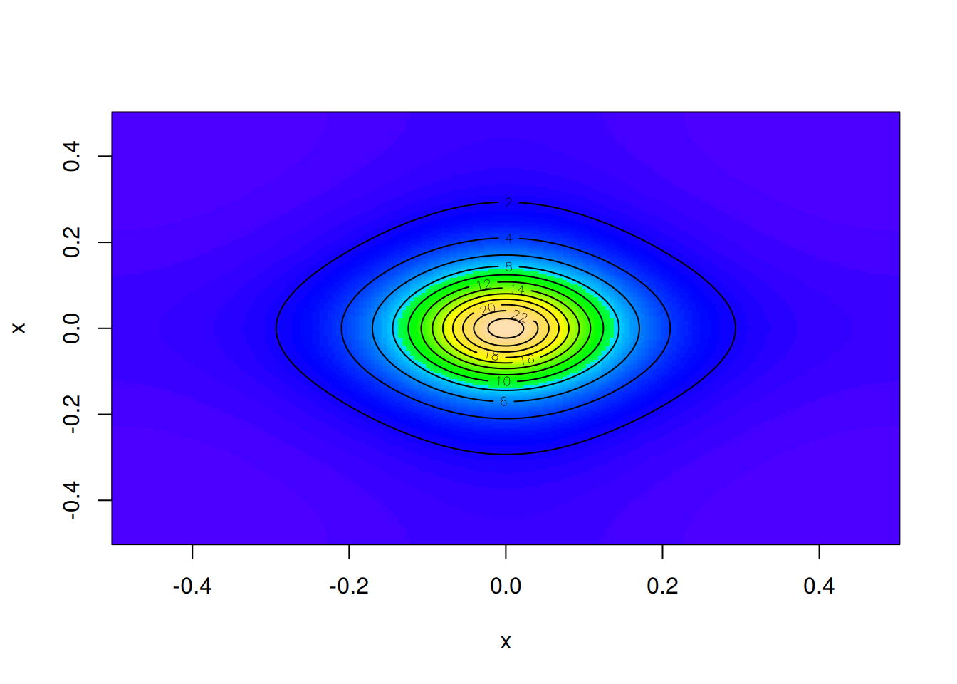
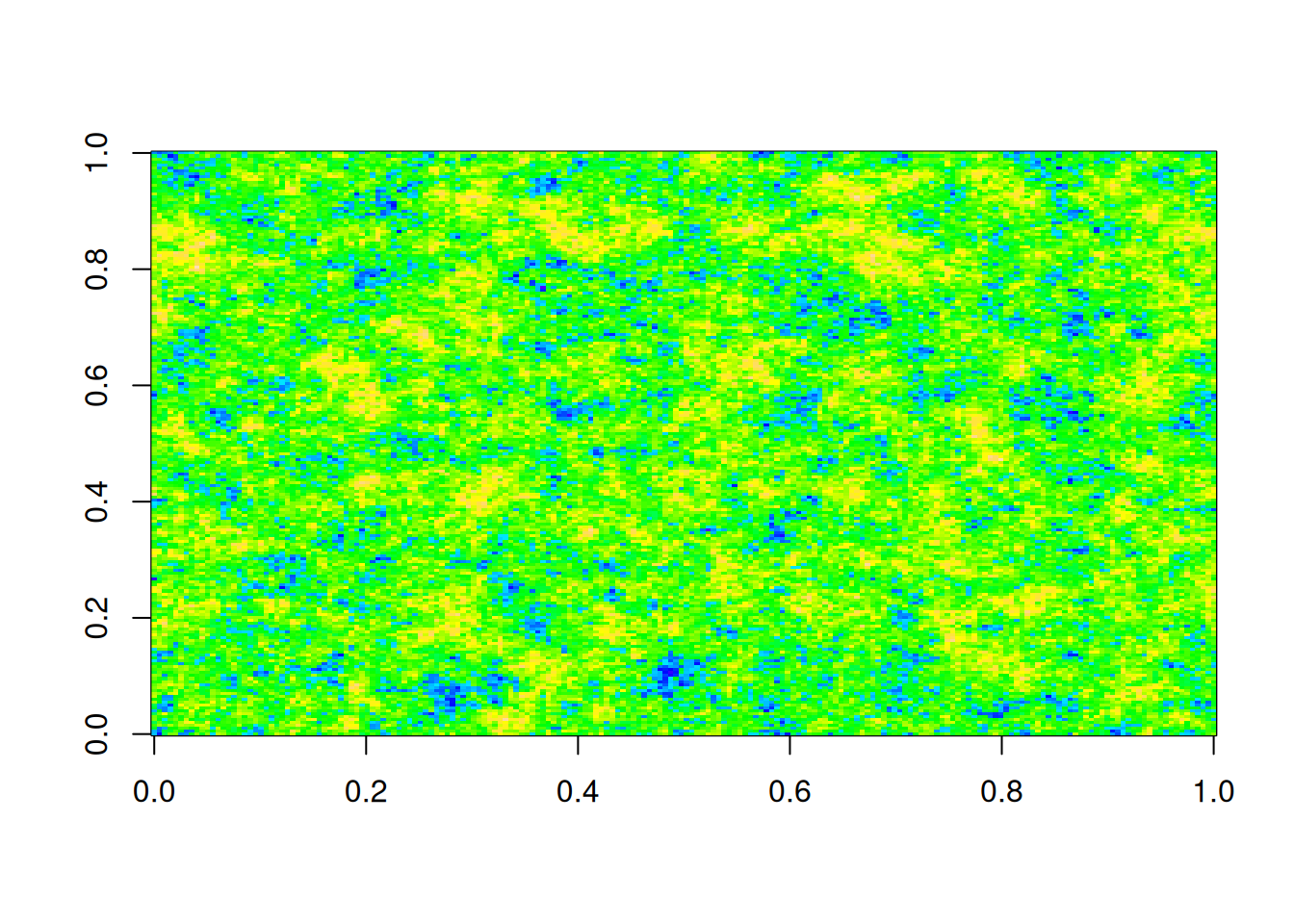
We can plot this spectrum in the case \(\alpha=\beta=1/5\), which clearly satisfies our stationarity condition.
We can see that for low frequencies (close to the centre of the plot), the contours are very circular, representing isotropic behaviour. However, as we move to higher frequencies the contours become distorted as the effects of the discrete lattice become more apparent.
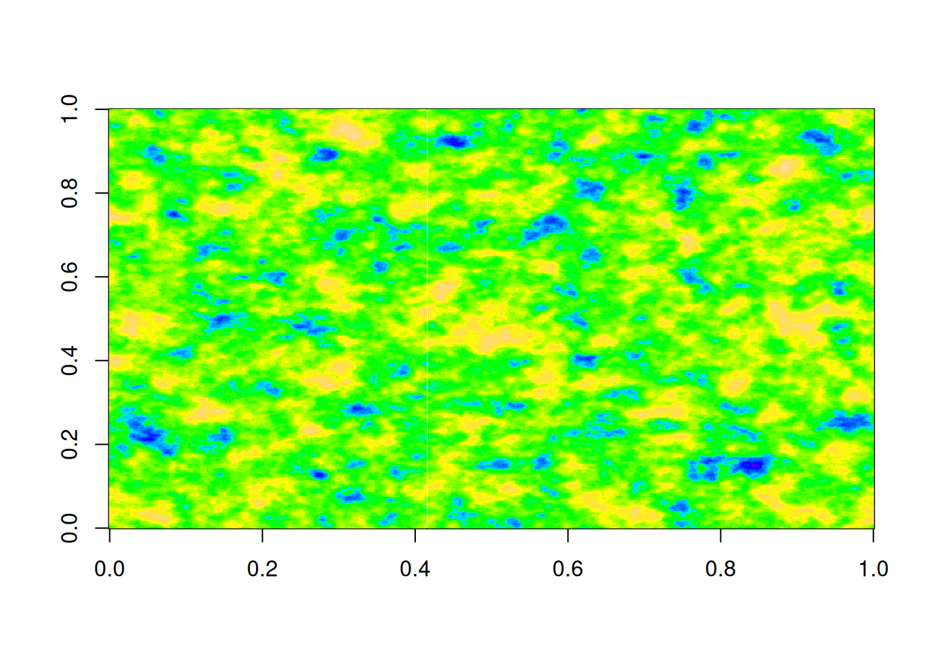
15.2.3 Simulation of stationary SAR models on a toroidal lattice
In practice we cannot work with infinite lattices. The closest we can do is work on a finite square lattice with periodic boundary conditions. This is equivalent to a toroidal lattice. In this case, the DFT of the model has a simple form allowing exact simulation, even for large lattices. We have the same model as just considered, \[
Z_{j,k} = \alpha(Z_{j+1,k}+Z_{j-1,k}) + \beta(Z_{j,k+1}+Z_{j,k-1}) + \varepsilon_{j,k},\quad \varepsilon_{j,k}\sim\mathcal{N}(0,\sigma^2).
\] But now \(j,k=0,1,\ldots,n-1\) and \(Z_{-j, k}=Z_{n-j, k}\), etc. In the case of periodic boundary conditions, the DFT of a shifted field again is simply related to the DFT of the unshifted field, so applying the 2d DFT to this model gives \[
[1-2\alpha\cos(2\pi l/n) - 2\beta\cos(2\pi m/n)]\hat{Z}_{l,m} = \hat{\varepsilon}_{l,m},\quad\text{where}\quad \hat{\varepsilon}_{l,m}\sim\mathcal{CN}(0,n^2\sigma^2).
\] In other words, \[
\hat{Z}_{l,m} = \frac{n\sigma}{1-2\alpha\cos(2\pi l/n) - 2\beta\cos(2\pi m/n)}\varepsilon'_{l,m},\quad \text{where}\quad \varepsilon'_{l,m}\sim\mathcal{CN}(0,1).
\] So we can just simulate this field in frequency space and invert. Again, the tricky bit is to ensure that all required conjugate symmetries are respected in order to get a real field. This is implemented below.
Since the FFT is extremely efficient, there’s no problem generating simulations on large lattices with \(\alpha\) and \(\beta\) close to the critical values.
As an alternative to using a simultaneous specification, we may prefer to specify a spatial model conditionally. Specifically, we may want to specify a set of local characteristics (or full conditional distributions) in order to fix a joint distribution over a random field. This is arguably more natural and intuitive than making a simultaneous specification. OTOH, we know that an arbitrary set of local characteristics may not be compatible with any joint distribution, and so care is required to ensure consistency with a proper model. To pursue the conditional specification approach, it will be extremely useful to have a simple way of determining the joint distribution associated with a particular set of local characteristics. The solution to this problem is typically referred to as Brook’s lemma.
Aside: this result is named after David Brook and/or Julian Besag, both of whom had strong connections to the North East of England. David worked for many years as a lecturer at Newcastle University. Julian was the Professor of Statistics at Durham University immediately before the appointment of Michael Goldstein. Shortly after leaving Durham, Julian was also briefly Professor of Statistics at Newcastle.
If \(\pi(\mathbf{x})\) is a density with \(\pi(\mathbf{x})>0\, \forall \mathbf{x}\in\mathcal{D}\subset\mathbb{R}^n\), then \(\forall \mathbf{x}, \mathbf{x}^\star \in \mathcal{D}\) we have \[\begin{align*}
\frac{\pi(\mathbf{x})}{\pi(\mathbf{x}^\star)}
&= \prod_{i=1}^n \frac{\pi(x_i|x_1,\ldots,x_{i-1},x_{i+1}^\star,\ldots,x_n^\star)}{\pi(x_i^\star|x_1,\ldots,x_{i-1},x_{i+1}^\star,\ldots,x_n^\star)} \\
&= \prod_{i=1}^n \frac{\pi(x_i|x_1^\star,\ldots,x_{i-1}^\star,x_{i+1},\ldots,x_n)}{\pi(x_i^\star|x_1^\star,\ldots,x_{i-1}^\star,x_{i+1},\ldots,x_n)} .
\end{align*}\]
Proof. We consider the case \(n=3\), from which generalisations should be clear. We start with \(\pi(\mathbf{x})\) and expand and simplify each variable in turn. Starting with \(x_1\) gives one equality and starting with \(x_n\) gives the other. We start with \(x_1\). \[\begin{align*}
\pi(\mathbf{x})
&= \pi(x_1,x_2,x_3) \\
&= \pi(x_1|x_2,x_3)\pi(x_2,x_3) \\
&= \pi(x_1|x_2,x_3)\frac{\pi(x^\star_1|x_2,x_3)}{\pi(x^\star_1|x_2,x_3)}\pi(x_2,x_3) \\
&= \frac{\pi(x_1|x_2,x_3)}{\pi(x^\star_1|x_2,x_3)}\pi(x^\star_1,x_2,x_3) \\
&= \frac{\pi(x_1|x_2,x_3)}{\pi(x^\star_1|x_2,x_3)}\pi(x_2|x^\star_1,x_3)\pi(x^\star_1,x_3) \\
&= \frac{\pi(x_1|x_2,x_3)}{\pi(x^\star_1|x_2,x_3)}\frac{\pi(x_2|x^\star_1,x_3)}{\pi(x^\star_2|x^\star_1,x_3)}\pi(x^\star_1,x^\star_2,x_3) \\
&= \frac{\pi(x_1|x_2,x_3)}{\pi(x^\star_1|x_2,x_3)}\frac{\pi(x_2|x^\star_1,x_3)}{\pi(x^\star_2|x^\star_1,x_3)}\pi(x_3|x^\star_1,x^\star_2)\pi(x^\star_1,x^\star_2) \\
&= \frac{\pi(x_1|x_2,x_3)}{\pi(x^\star_1|x_2,x_3)}\frac{\pi(x_2|x^\star_1,x_3)}{\pi(x^\star_2|x^\star_1,x_3)}\frac{\pi(x_3|x^\star_1,x^\star_2)}{\pi(x^\star_3|x^\star_1,x^\star_2)}\pi(\mathbf{x}^\star)
\end{align*}\]
This result allows us to pick a convenient reference state, \(\mathbf{x}^\star\) (often \(\mathbf{x}^\star=\mathbf{0}\) is used), and then write the joint distribution for \(\mathbf{x}\), up to a normalising constant, as a product of ratios of full-conditionals.
15.3.1.1 Example: AR(1)
Returning to our example of a pair of values from an AR(1), we can use Brook’s lemma to expand the joint distribution in two different ways (using reference state \(\mathbf{x}^\star=\mathbf{0}\), and dropping terms not involving \(x\) or \(y\)), \[
f_{X,Y}(x,y) \propto f_{X|Y}(x|0)\frac{f_{Y|X}(y|x)}{f_{Y|X}(0|x)},
\] and \[
f_{X,Y}(x,y) \propto \frac{f_{X|Y}(x|y)}{f_{X|Y}(0|y)}f_{Y|X}(y|0).
\] Substituting in our two conditional distributions and simplifying leads to the same joint distribution (bivariate normal with variances \(\sigma^2/(1-\alpha^2)\) and correlation \(\alpha\)).
15.3.2 CAR model specification
A (Gaussian) CAR model for the joint distribution over \(n\) spatial locations is specified via a normal local characteristic (full-conditional distribution) at each site. \[
(Z_i|\mathbf{Z}_{-i}=\mathbf{z}_{-i}) \sim \mathcal{N}\left( \sum_{j=1}^n a_{ij}z_j, \kappa_i \right),\quad i=1,2,\ldots,n.
\] It is assumed that \(\kappa_i>0\) and \(a_{ii}=0,\ \forall i\). The coefficients, \(a_{ij}\) can be stored in the \(n\times n\) matrix \(\mathsf{A}\) with zero diagonal. The non-zero elements of \(\mathsf{A}\) represent some kind of neighbourhood structure (to be made precise soon). We expect that most \(a_{ij}\) will be 0, so \(\mathsf{A}\) will be a sparse matrix. It will also turn out to be convenient to define \(\mathsf{K}=\operatorname{diag}\{\kappa_i\}\). Some care is needed to ensure that the local characteristics are actually compatible with a proper joint distribution. We want to identify the joint distribution and any necessary constraints on the elements of \(\mathsf{A}\) and \(\mathsf{K}\).
15.3.3 Joint distribution
We could just use Brook’s lemma (with reference state \(\mathbf{x}^\star=\mathbf{0}\)) to directly compute the joint density (up to a normalising constant), recognising the multivariate normal distribution that arises. Doing this is left as an exercise. Instead, we will guess that the joint distribution will be of the form \[
\mathbf{Z} \sim \mathcal{N}(\mathbf{0},\mathsf{Q}^{-1}),
\] for some (presumably sparse) precision matrix, \(\mathsf{Q}\). By comparing the full-conditionals of this multivariate normal with our CAR local characteristics, we can identify the relationship between \(\mathsf{A}\), \(\mathsf{K}\) and \(\mathsf{Q}\).
Using our results for multivariate normal conditioning based on a partitioned precision matrix, from Section 14.2.4, we find that the full-conditionals are \[
(Z_i|\mathbf{Z}_{-i}=\mathbf{z}_{-i}) \sim \mathcal{N}\left(-\frac{1}{q_{ii}}\sum_{j\not= i} q_{ij}z_j, \frac{1}{q_{ii}} \right).
\] Comparing against our CAR local characteristic specifications, we see that we must have \[
q_{ii} = \frac{1}{\kappa_i},\quad \forall i,
\] and \[
-\frac{q_{ij}}{q_{ii}} = a_{ij} \quad \Rightarrow \quad q_{ij} = -\frac{a_{ij}}{\kappa_i},\quad \forall i\not= j.
\] This fully specifies \(\mathsf{Q}\). In matrix form, \[
\mathsf{Q} = \mathsf{K}^{-1}(\mathbb{I}-\mathsf{A}),
\] since pre-multiplication by a diagonal matrix corresponds to re-scaling the rows. This reveals some constraints that our specification must satisfy for a joint distribution to exist. First, since the precision matrix is symmetric, we must have \(q_{ij}=q_{ji}\), and therefore we must have \[
\frac{a_{ij}}{\kappa_i} = \frac{a_{ji}}{\kappa_j}, \quad \forall i,j.
\] Further, since the precision matrix is positive definite, \(\mathsf{K}^{-1}(\mathbb{I}-\mathsf{A})\) must be positive definite. So, our constraints can be summarised as: \[
\mathsf{K}^{-1}(\mathbb{I}-\mathsf{A})
\]must be symmetric and positive definite. Then, \[
\mathbf{Z} \sim \mathcal{N}(\mathbf{0},(\mathbb{I}-\mathsf{A})^{-1}\mathsf{K}).
\] We will need to ensure that any CAR model specification respects these constraints. Provided that we have a consistent model, its properties are quite intuitive. Since \(\mathsf{K}\) simply re-scales the rows, the sparsity structure of \(\mathsf{Q}\) and \(\mathbb{I}-\mathsf{A}\) are the same. So the non-diagonal sparsity of \(\mathsf{Q}\) and \(\mathsf{A}\) are the same. That is, the (off-diagonal) zeros in \(\mathsf{A}\) correspond to zeros in \(\mathsf{Q}\), and therefore pairwise conditional independence properties. In other words, the zero structure of \(\mathsf{A}\) determines the conditional independence structure of the implied GGM.
15.3.3.1 Equal weight specification
Very often we will want to define a CAR model on a graph with unweighted edges. In this case, we typically want each node to depend equally on its neighbours. It is therefore natural to specify \[
a_{ij} = \begin{cases}
\displaystyle
\frac{\rho}{n_i}, & \mathbf{s}_i \sim \mathbf{s}_j \\
0 & \text{otherwise},
\end{cases}
\] where \(n_i\) is the number of neighbours of site \(i\), and \(\rho\in(0,1)\) is a dependence parameter ensuring that the total weight assigned to node \(i\), \(\rho\), does not exceed one (required for diagonal dominance of \(\mathbb{I}-\mathsf{A}\), ensuring invertibility). Values of \(\rho\) close to one will be associated with high spatial dependence. Setting \(\rho=1\) gives an improper CAR prior, which we are not discussing here.
We might like to set \(\kappa_i\) to a constant value, \(\kappa\), but for an irregular graph with varying numbers of node neighbours this would violate our required consistency condition. Instead we must choose \[
\kappa_i = \frac{\kappa}{n_i}, \quad \forall i,
\] for some fixed \(\kappa>0\), since then \[
\frac{a_{ij}}{\kappa_i} = \frac{\rho/n_i}{\kappa/n_i} = \frac{\rho}{\kappa} = \frac{\rho/n_j}{\kappa/n_j} = \frac{a_{ji}}{\kappa_j},
\] and our consistency requirement is satisfied. Note that in addition to being required for consistency, this assumption for the conditional variance is often quite reasonable, since it is quite natural to think that the more information you have from neighbouring sites, the less residual uncertainty you will have about the current site.
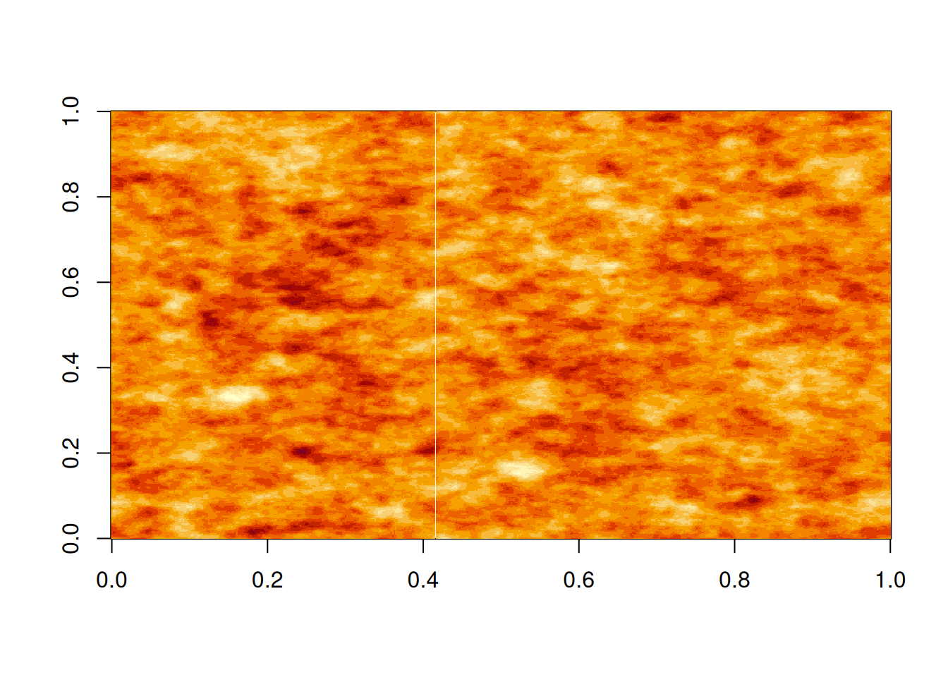
15.3.4 Spectrum of a CAR model on a regular lattice
If we call the variance matrix \(\mathsf{\Sigma}\), the previous section has demonstrated that \[
(\mathbb{I}-\mathsf{A})\mathsf{\Sigma} = \mathsf{K},
\] which we can regard as a set of \(n^2\) linear equations for the elements of \(\mathsf{\Sigma}\). Explicitly, if we let \(c_{ij}\) be the \((i,j)\)th element of \(\mathsf{\Sigma}\), then the \((i,j)\)th equation is \[
c_{ij} - \sum_k a_{ik}c_{jk} = \kappa_i\delta_{ij}.
\] These equational relations are more convenient in the case of infinitely many sites.
We can now consider a stationary CAR model specification on an infinite regular square lattice. The local characteristic at position \(\mathbf{s}=(j,k)\) is \[
Z_{j,k}|\mathbf{Z}_{-(j,k)} \sim \mathcal{N}(\alpha[Z_{j-1,k}+Z_{j+1,k}]+\beta[Z_{j,k-1}+Z_{j,k+1}],\kappa),
\] assuming that the conditional variance, \(\kappa\), is constant, which is fine here, since every node has the same number of neighbours. Our infinite set of equations for the covariogram \(C(\mathbf{h})=C(j,k)=\mathbb{C}\mathrm{ov}[Z_{l,m},Z_{l+j,m+k}]\) are of the form \[
C(j,k) -\alpha[C(j-1,k)+C(j+1,k)]-\beta[C(j,k-1)+C(j,k+1)]=\kappa\delta_j\delta_k.
\] These are the equivalent of the Yule-Walker equations for a CAR model on a square lattice. We can Fourier transform these covariance relations in order to get an equation for the spectrum. \[\begin{align*}
S(\pmb{\nu}) - \alpha[e^{-2\pi\mathrm{i}\nu_x}+e^{2\pi\mathrm{i}\nu_x}]S(\pmb{\nu}) - \beta[e^{-2\pi\mathrm{i}\nu_y} + e^{2\pi\mathrm{i}\nu_y}]S(\pmb{\nu}) &= \kappa \\
\Rightarrow [1-2\alpha\cos(2\pi\nu_x)-2\beta\cos(2\pi\nu_y)]S(\pmb{\nu}) &=\kappa,
\end{align*}\] and so \[
S(\nu) = \frac{\kappa}{1-2\alpha\cos(2\pi\nu_x)-2\beta\cos(2\pi\nu_y)}.
\] This is similar to, but importantly different from, the corresponding spectrum of the nearest neighbour SAR model. Again, we want \(\alpha+\beta < 1/2\) for stationarity (assuming \(\alpha,\beta>0\)). Comparing back with the spectra we computed for AR(\(p\)) models, this CAR spectrum is more “AR(1)-like”, whereas the SAR spectrum is more “AR(2)-like”.
15.3.5 Simulation of CAR models
Since the CAR model specification corresponds to a multivariate normal distribution, in principle we can generate realisations of the CAR process using standard methods for simulating from a multivariate normal. However, if the number of sites is large and/or the lattice is regular, then there may be better approaches.
15.3.5.1 Spectral synthesis on a toroidal lattice
If we are working on a finite square lattice and are happy to assume periodic boundary conditions (ie. assume a toroidal lattice), then we can simulate very efficiently using the FFT. We can apply the DFT to our covariance relations, noting that the DFT of \(C(j,k)\) is actually \(S_{l,m}/n^2\) (annoying factors of \(n\)), where \(S_{l,m}\) is the spectral density at frequencies \(l\) and \(m\), to get \[\begin{align*}
\frac{S_{l,m}}{n^2} - \alpha[e^{-2\pi\mathrm{i}l/n} + e^{2\pi\mathrm{i}l/n} ]\frac{S_{l,m}}{n^2} - \beta[e^{-2\pi\mathrm{i}m/n}+e^{2\pi\mathrm{i}m/n}]\frac{S_{l,m}}{n^2} &= \kappa \\
\Rightarrow [1-2\alpha\cos(2\pi l/n)-2\beta\cos(2\pi m/n)]S_{l,m} &= n^2\kappa,
\end{align*}\] and so \[
S_{l,m} = \frac{n^2\kappa}{1-2\alpha\cos(2\pi l/n)-2\beta\cos(2\pi m/n)}.
\] Then, we can use our spectral synthesis approach to generate realisations using the FFT. As usual, the fiddly bit is respecting the required conjugate symmetries.
Away from the very special case of a stationary field on a toroidal lattice, things are not so convenient. We know that \[
\mathbf{Z} \sim \mathcal{N}(\mathbf{0}, \mathsf{Q}^{-1}), \quad \text{where} \quad \mathsf{Q} = \mathsf{K}^{-1}(\mathbb{I}-\mathsf{A}),
\] and \(\mathsf{Q}\) will typically be a very sparse matrix. However, \(\mathsf{\Sigma}=\mathsf{Q}^{-1}\) typically will not be very sparse, so we would like to be able to simulate realisations of the field using \(\mathsf{Q}\) directly and without constructing \(\mathsf{\Sigma}\). It is actually quite straightforward to do this. First, form the Cholesky decomposition of \(\mathsf{Q}\) as \[
\mathsf{Q} = \mathsf{L}\mathsf{L}^\top,
\] where \(\mathsf{L}\) is a lower triangular matrix. If \(\mathsf{Q}\) is sparse, then \(\mathsf{L}\) will typically also be sparse, though typically not as sparse as \(\mathsf{Q}\). The additional non-zero entries in the lower triangle of \(\mathsf{L}\) are known as fill-in. The level of fill-in depends heavily on the ordering of the rows and columns of \(\mathsf{Q}\), and so fill-reducing permutations can be applied to \(\mathsf{Q}\) prior to computing the Cholesky decomposition in order to maintain as much sparsity as possible. Once we have \(\mathsf{L}\), we can generate \(\varepsilon_i\sim\mathcal{N}(0,1)\) and solve the upper triangular linear system \[
\mathsf{L}^\top\mathbf{Z} = \pmb{\varepsilon}
\] for \(\mathbf{Z}\) using backward substitution. Backward substitution can be implemented very efficiently for sparse systems. The resulting \(\mathbf{Z}\) vector has exactly the distribution we want, since \[
\mathbb{V}\mathrm{ar}[\mathbf{Z}] = \mathbb{V}\mathrm{ar}[(\mathsf{L}^\top)^{-1}\pmb{\varepsilon}] = (\mathsf{L}^\top)^{-1}\mathbb{V}\mathrm{ar}[\pmb{\varepsilon}]\mathsf{L}^{-1}= (\mathsf{L}^\top)^{-1}\mathsf{L}^{-1}= \mathsf{Q}^{-1}=\mathsf{\Sigma},
\] as required.
For large systems, we will want to use specialised sparse matrix algorithms (such as provided by the R Matrix package), but for smaller systems we can follow the above recipe using standard dense algorithms. This will still be more numerically stable than attempting to simulate via direct inversion of \(\mathsf{Q}\).
15.3.5.3 Example: CAR model for NC counties
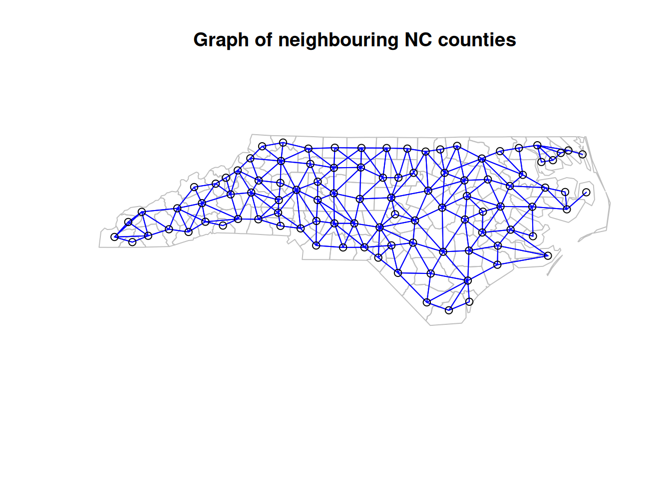
We will now illustrate exact simulation from an equally weighted CAR specification on an irregular graph using the example of counties in North Carolina (NC). Since there are only 100 counties, the precision matrix will only be \(100\times 100\), and so we don’t need to worry about using sparse matrix libraries.
Let us begin by loading the data and reminding ourselves of the neighbourhood structure.
The object ncCR85_nb is a neighbour list. This can be used to construct sparse or dense adjacency and weight matrices. Here we can just form dense matrices.
adj=nb2mat(ncCR85_nb, style="B")# binary adjacency matrixadjW=nb2mat(ncCR85_nb)# weight matrix with rows summing to oneprint(dim(adj))
Once we have the precision matrix, we can generate an exact sample from the CAR model.
Lt=chol(Q)# upper Cholesky triangleset.seed(57)z=backsolve(Lt, rnorm(n))# solve using backward substitution
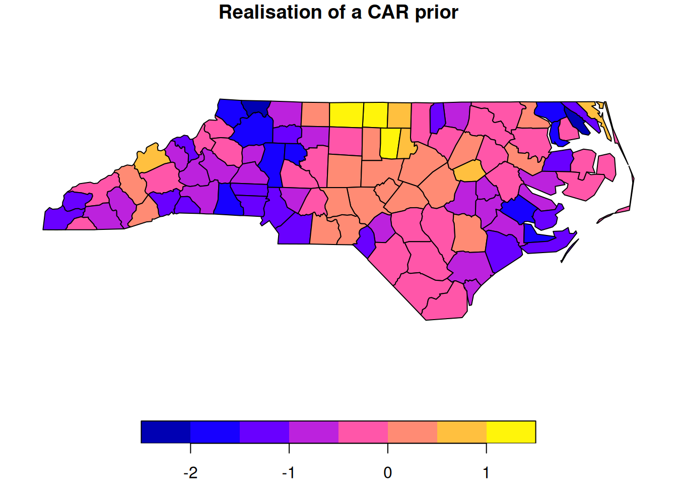
We can add this sample as an additional column to the nc spatial data frame and then plot it.
nc["car"]=z# add CAR sample to spatial data frameplot(nc["car"], main="Realisation of a CAR prior")
We see that this random sample from the CAR model has exactly the properties that we would want. It is random, but with a high degree of spatial dependence, so that neighbouring counties are much more highly correlated than distant counties.
15.3.5.4 Gibbs sampling
The Gibbs sampler is an especially convenient way to generate approximate samples from a CAR model. The Gibbs sampler is a special case of a more general class of techniques known as Markov chain Monte Carlo (MCMC). These methods are concerned with simulating Markov chains with a stationary equilibrium distribution equal to a (complicated, high-dimensional) target of interest. The Gibbs sampler is based on the observation that sampling from a full-conditional distribution of a given distribution will leave the target invariant. Therefore, cycling through each full-conditional in turn and sampling from it will typically give an ergodic Markov chain with the required equilibrium. Since a CAR model is specified in terms of its full-conditional distributions, Gibbs sampling CAR models is especially simple and convenient, and is arguably one of the reasons for the popularity of the CAR specification. Unfortunately, we don’t have time to explore this in detail in this course.
15.4 Comparing SAR and CAR
Both SAR and CAR models give rise to multivariate Gaussian distributions with a sparse conditional independence structure, so it is worth contemplating the relative merits of the two modelling approaches. Ultimately, it is a modelling preference: CAR will be more natural if you “think conditionally” and SAR will be more natural if you “think simultaneously”. However, the very close connection between the conditional specification underlying CAR and the undirected conditional independence graph of the model is a compelling reason to prefer CAR for many people. The CAR specification is often also more convenient computationally, especially in the context of MCMC algorithms, as discussed above.
Another reason to prefer CAR is that it is more general. Every SAR model can be written as a CAR model, but there are CAR models that can not be expressed as a SAR. To better understand this, equate the precision matrices for the two models, \[
\mathsf{Q} = (\mathbb{I}-\mathsf{B}^\top)\mathsf{\Lambda}^{-1}(\mathbb{I}-\mathsf{B}) = \mathsf{K}^{-1}(\mathbb{I}-\mathsf{A}) .
\] It is clear that the \(\mathsf{Q}\) arising from any model can be decomposed into a CAR model specification by taking \(\mathsf{K}^{-1}\) to be the diagonal of \(\mathsf{Q}\) and then solving for \(\mathsf{A}\). Conversely, it is not difficult to construct examples of CAR model specifications which can not be factored into the form of a SAR model.
All this said, simultaneous equations models (SEMs) are very widely used in economics and related fields. SAR models are essentially spatial SEMs, and hence are popular with people from this kind of background.
15.5 Auto-models
The SAR and CAR models that we have studied are both methods for building multivariate normal distributions with interesting covariance structures. Things get a lot more complicated once we move away from the Gaussian case. Auto-models are a generalisation of the CAR models we have been thinking about, where now the local characteristics are allowed to be from the exponential family. Since the Gaussian distribution is from the exponential family, this generalisation is quite natural. To better understand auto-models, it will helpful to view them as Gibbs random fields. For MRFs on a square lattice, only pairwise interactions are possible, so the Gibbs potential will be of the form \[
V(\mathbf{x}) = \sum_{i,j:i<j,i\sim j} \psi_{i,j}(x_i,x_j).
\] For a GMRF, the local potential functions will be quadratic in \(x_i,x_j\). But since they are quadratic, all interactions are pairwise for a GMRF, irrespective of the topology of the lattice, since the cross terms are all of the form \(\beta_{i,j}x_ix_j\) (for some \(\beta_{i,j}=\beta_{j,i}\)). It is therefore natural to restrict attention to models with only pairwise interactions, since we know that these already provide us with a very rich structure. In fact, it will turn out to be convenient to keep precisely the form of the cross terms found in a GMRF, and propose a potential of the form \[
-V(\mathbf{x}) = \sum_i x_i G_i(x_i) + \sum_{i,j:i<j,i\sim j} \beta_{i,j}x_ix_j,
\] for some given functions \(G_i(\cdot)\). Clearly, if we choose the \(G_i(\cdot)\) to be linear, then we will get a quadratic potential, and a GMRF. But now we generalise beyond the GMRF, and consider other functions.
By definition, the joint density of the random field will be of the form \[
\pi(\mathbf{x}) \propto \exp\{-V(\mathbf{x})\},
\] and once we move away from the Gaussian case, the normalising constant of the density will typically be intractable. This complicates the use of such models for inference. Nevertheless, we can compute the local characteristics as \[
\pi(x_i|\mathbf{x}_{-i}) \propto \exp\left\{x_iG_i(x_i)+\sum_{j:j\sim i}\beta_{i,j}x_ix_j\right\}.
\] It is then clear that our simple choice of cross term ensures that our local characteristics are exponential family wrt the interaction parameters. This is useful for both theoretical and practical reasons. Recall that the exponential family covers a range of discrete and continuous distributions, so this formalism opens up the possibility of defining distributions on fields with different kinds of support.
15.5.1 Auto-logistic/Ising model
It is sometimes desirable to be able to define MRFs where the value of the field at each node is binary, usually (in statistics) assumed to be 0 or 1. But if \(x_i\) is binary, then the term \(x_iG_i(x_i)\) can only take on two distinct values, irrespective of the choice of function, and hence we may as well assume \(G_i(x_i) = \alpha_i\), a constant function. Then we have \[
-V(\mathbf{x}) = \sum_i \alpha_i x_i + \sum_{i,j:i<j,i\sim j} \beta_{i,j}x_ix_j,
\] and hence joint probability mass function, \[
\pi(\mathbf{x}) \propto \exp\left\{ \sum_i \alpha_i x_i + \sum_{i,j:i<j,i\sim j} \beta_{i,j}x_ix_j \right\}.
\] If we are working on a finite lattice with \(n\) nodes, we might imagine that we can deduce the normalising constant of this distribution by summing over all possible states of the system. Although this is possible in principle, there are \(2^n\) different possible configurations of this model, and so for non-trivial \(n\), the normalising constant is intractable for all practical purposes. Nevertheless, the local characteristics are completely tractable. Up to a constant of proportionality we have \[
\pi(x_i|\mathbf{x}_{-i}) \propto \exp\left\{\alpha_i x_i+\sum_{j:j\sim i}\beta_{i,j}x_ix_j\right\},
\] but since \(x_i\) is binary it is trivial to sum over the possible states to obtain the normalising constant. This then gives the local characteristic as Bernoulli, \(\text{Bern}(p_i)\) with \[
p_i = \frac{\exp\left\{\alpha_i +\sum_{j:j\sim i}\beta_{i,j}x_j\right\}}{1+\exp\left\{\alpha_i +\sum_{j:j\sim i}\beta_{i,j}x_j\right\}} = \frac{1}{1+\exp\left\{-\alpha_i -\sum_{j:j\sim i}\beta_{i,j}x_j\right\}}.
\] By this point it should be clear why this is known as the auto-logistic model. It should also be clear that whilst we can’t easily simulate exact realisations from this process, it is very simple to use a Gibbs sampler to construct a Markov chain having this model as its equilibrium distribution.
Although we have motivated the development of this model from a spatial statistics perspective, it also crops up as a model of ferromagnetism in statistical mechanics, where it is known as the Ising model. There are many different ways to parameterise this model, some of which look quite different.
Consider a model for a binary-valued Gibbs random field with potential function \[
-V(\mathbf{x}) = \psi\sum_{i,j:i<j,i\sim j} w_{ij}\mathbb{I}(x_i=x_j),
\] where \(\mathbb{I}(x_i=x_j)\) is 1 if \(x_i=x_j\) and 0 otherwise (essentially Kronecker’s delta). We can now observe that when \(x_i,x_j\in\{0,1\}\), we have \[\begin{align*}
\mathbb{I}(x_i=x_j) &= x_i x_j + (1-x_i)(1-x_j)\\
&= 1-x_i-x_j+2x_ix_j,
\end{align*}\] and substituting this back into our potential function reveals that this is really just our auto-logistic model in disguise. However, this way of parameterising the model is arguably more insightful. Up to a constant of proportionality, the local characteristics of this model are \[
\pi(x_i|\mathbf{x}_{-i}) \propto \exp\left\{\psi\sum_{j:j\sim i} w_{ij}\mathbb{I}(x_i=x_j)\right\}.
\] So we see that locally, the probability of a node being in a certain state depends on which neighbours are in the same state. In particular, if \(\psi\) and \(w_{ij}>0\), then the probability of being in a given state increases with the number of neighbours in the same state. This then gives rise to positive spatial dependence, with nearby nodes being more likely to be in the same state than nodes far apart. Normalising this gives the local characteristic as \(\text{Bern}(p_i)\) with \[
p_i = \frac{1}{1+\exp\left\{-\psi\sum_{j:j\sim i} w_{ij}[\mathbb{I}(x_j=1)-\mathbb{I}(x_j=0)]\right\}}.
\]
15.5.2 Potts model
The Ising model is a binary-valued Gibbs random field. In the context of spatial statistics, this is useful when trying to make inferences about a hidden process that is binary. One example of this would be binary image segmentation, where each image pixel is to be classified into one of two categories. For example, in the context of microscopy, the classification might be 1 for a pixel that is part of a cell nucleus and 0 otherwise. But in some cases we might want to segment an image (or other lattice field) into more than two categories. The natural generalisation of the Ising model to \(K\in\mathbb{N}\) categories is known (to physicists) as the Potts model. When used as the hidden state of an image segmentation model, it becomes the spatial analogue of the hidden Markov model we used for time series and sequence analysis.
Suppose now that the random field can take on \(K\) possible values, say, \(x_i\in\{0,1,\ldots,K-1\}\). We can (again) define the joint density via, \[
\pi(\mathbf{x}) \propto \exp\left\{ \psi\sum_{i,j:i<j,i\sim j} w_{ij}\mathbb{I}(x_i=x_j) \right\},
\] where now the normalising constant is a sum over all \(K^n\) possible states, and hence is even more intractable than that of the Ising model. The local characteristics are, up to a constant of proportionality, \[
\pi(x_i|\mathbf{x}_{-i}) \propto \exp\left\{\psi\sum_{j:j\sim i} w_{ij}\mathbb{I}(x_i=x_j)\right\},
\] just as for the Ising model. This model then clearly also has the property that the probability of being in a given state will depend on the number of neighbours that are in the same state. We can normalise the local characteristics to get a discrete distribution on \(x_i\in\{0,1,\ldots,K-1\}\) as \[
\mathbb{P}(x_i=k|\mathbf{x}_{-i}) = \frac{\displaystyle\exp\left\{\psi\sum_{j:j\sim i} w_{ij}\mathbb{I}(k=x_j)\right\}}{\displaystyle\sum_{k'=0}^{K-1}\exp\left\{\psi\sum_{j:j\sim i} w_{ij}\mathbb{I}(k'=x_j)\right\}}.
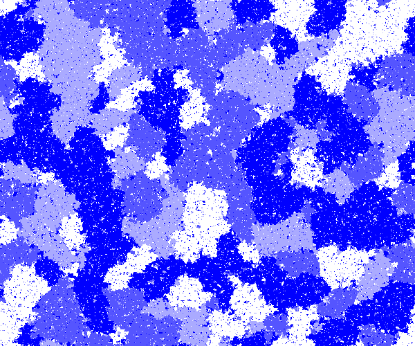
\] For large \(n\) it is essentially impossible to directly simulate exact realisations from this model, but it is very straightforward to use a Gibbs sampler to generate MCMC samples. Below is a realisation of a Potts model on a \(600\times 500\) regular square lattice, generated using a Gibbs sampler, with \(K=4\) states shown as different shades of blue.
A realisation from a Potts model on a square lattice with 4 states.