Load up RStudio via your favourite method. If you can’t use RStudio for some reason, most of what we do in these labs can probably be done using WebR, but the instructions will assume RStudio. You will also want to have the web version of the lecture notes to refer to.
Question 1
If you haven’t already done so, reproduce all of the plots and computations from Chapter 16 of the lecture notes by copying and pasting each code block in turn. Make sure you understand what each block is doing and that you can reproduce all of the plots.
Question 2
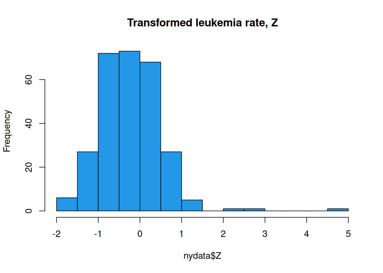
Today we will be again using the New York, spData::nydata. We will focus on the actual data of interest, relating to incidence rate of leukemia in the population, Z. First, load some libraries and look at the data.
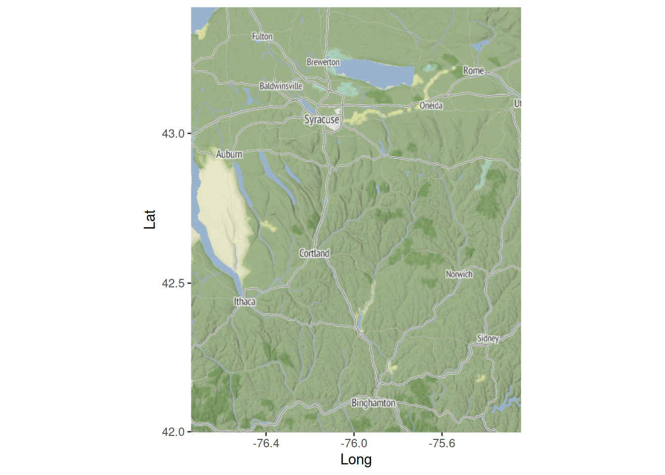
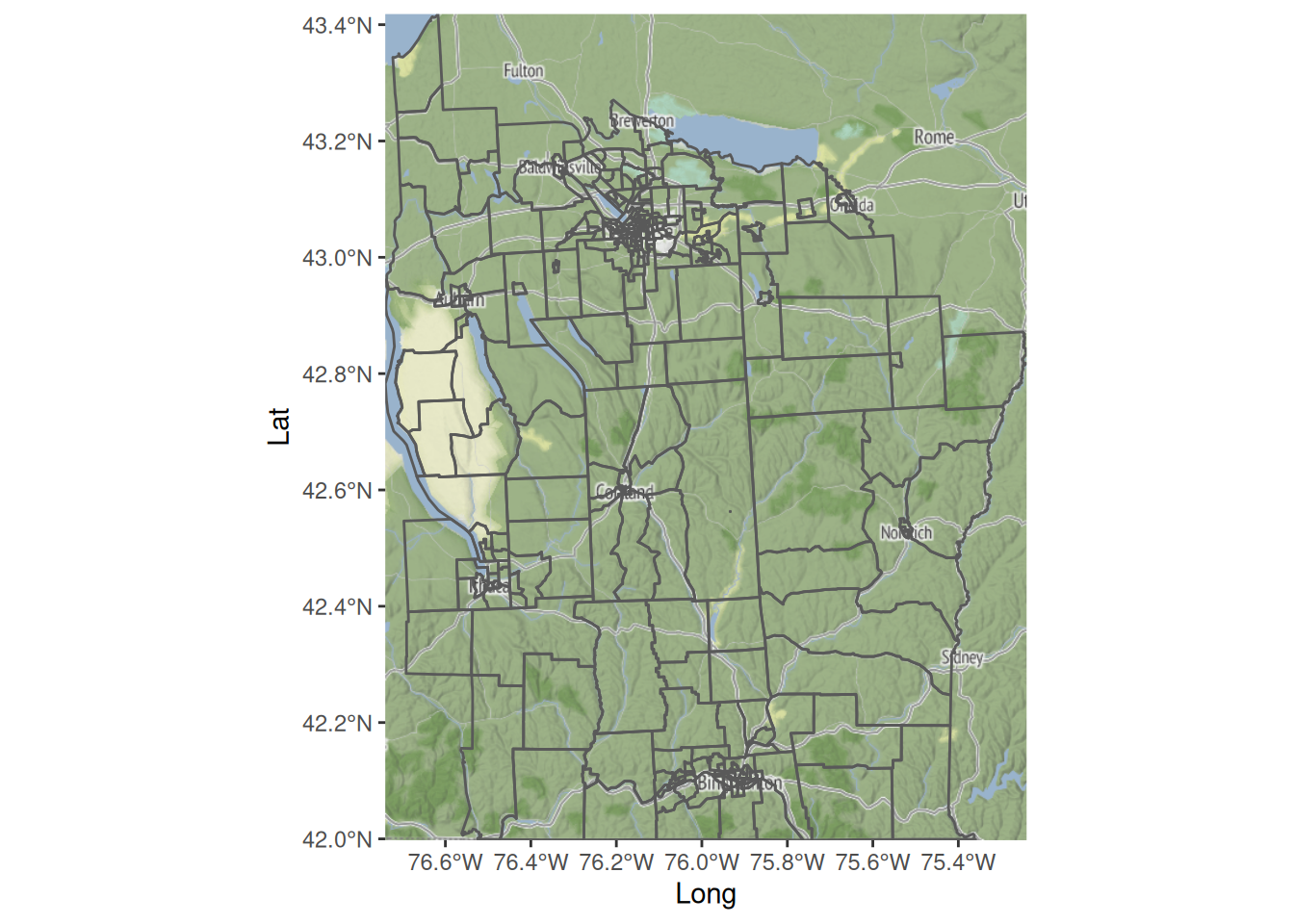
If you have a StadiaMaps API key, you can view the spatial context of the data. If you don’t have an API key, skip the next two code blocks. They are not required for what follows. We can start with a plain map of the region.
nyd_ll=st_transform(nyd, "EPSG:4326")# long and latnyd_bb=st_bbox(nyd_ll)names(nyd_bb)=c("left", "bottom", "right", "top")nyd_map=get_map(nyd_bb, maptype="stamen_terrain", source="stadia")ggmap(nyd_map)+labs(x="Long", y="Lat")
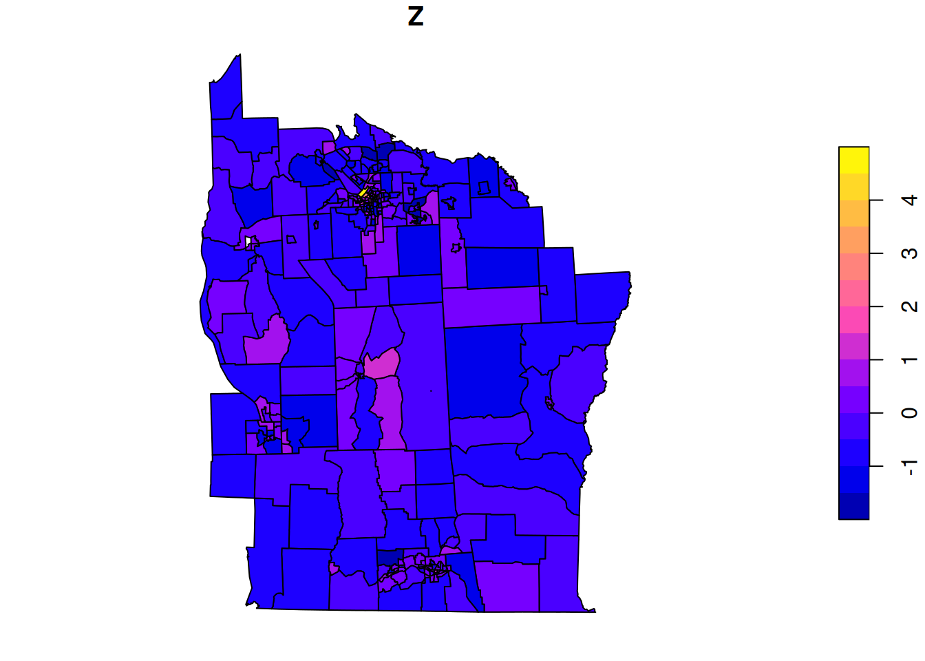
So we see that the data relates to part of New York State (rather than New York City), and that the biggest city in the region covered by the data is Syracuse, NY, which also seems to be associated with the highest rates of Leukemia.
Let us now investigate spatial modelling of the leukemia rate, Z.
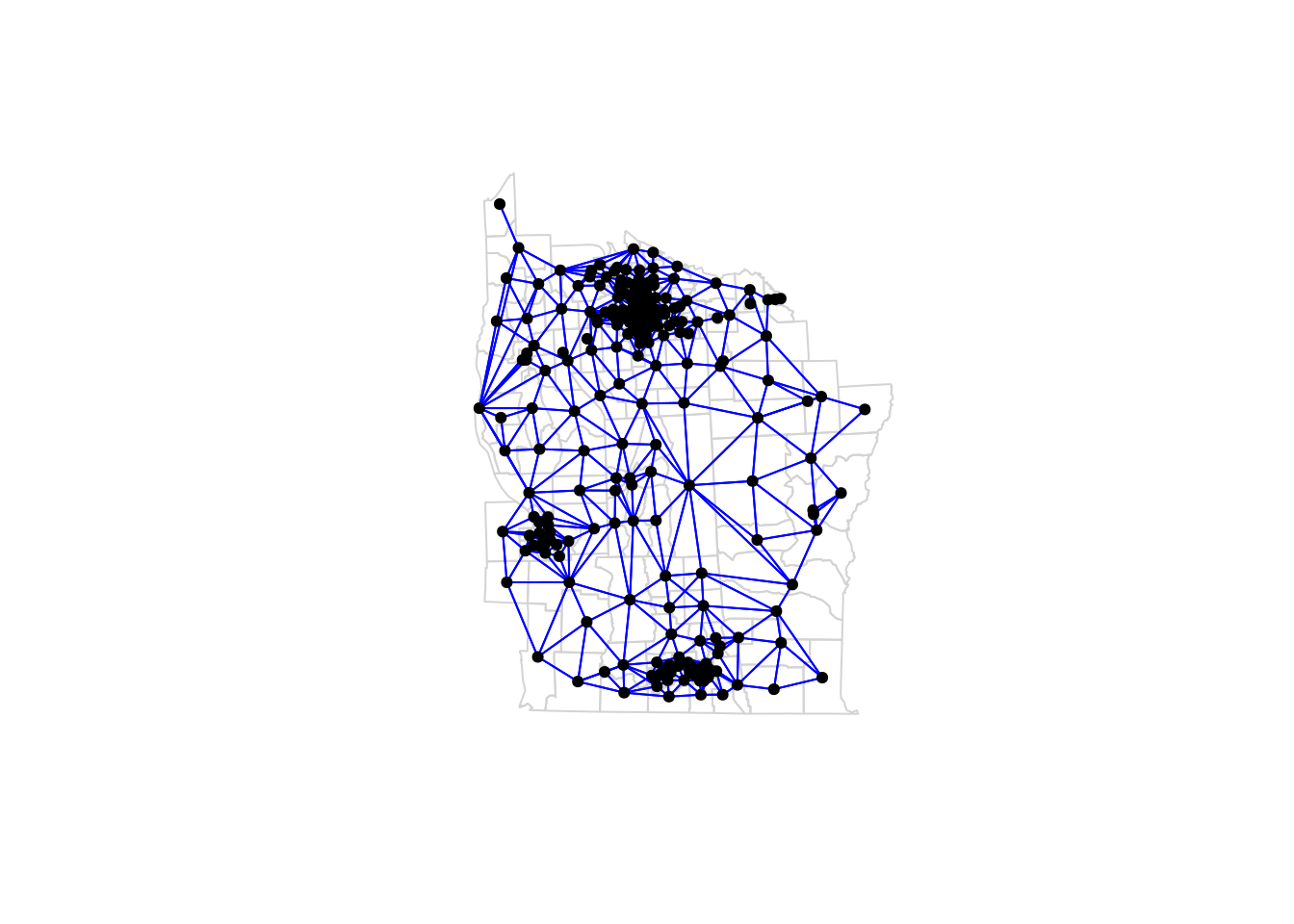
Hopefully you detected the presence of spatial association. Let’s begin with some spatial smoothing of the data. We need a spatial prior, and the only examples we know much about are SAR and CAR. Let’s start with an equally weighted SAR model. First set up an appropriate normalised adjacency matrix.
We will use this to construct a SAR prior using a spatial dependency parameter of 0.999, and a residual variance of 0.2. Note that we could have a residual variance that is dependent on the number of neighbours, as we have to with CAR, but since we don’t have to for SAR, let’s not bother.
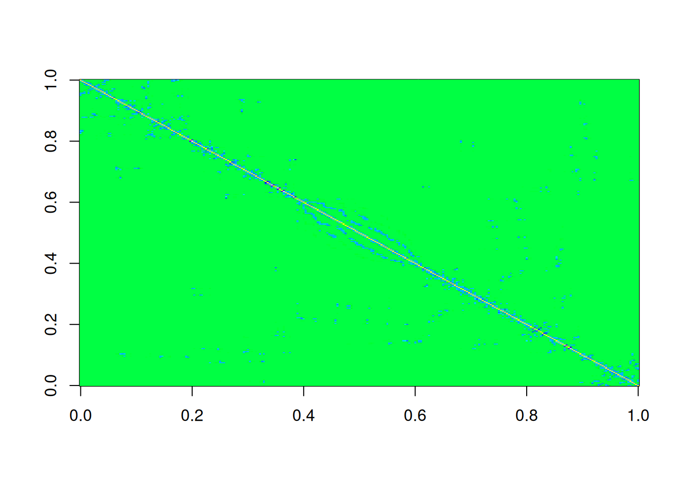
sigma=0.2# residual errorrho=0.999# spatial dependence parameter (< 1 for diagonal dominance)B=adjW*rho# sensible SAR weight matrixQ=(1/(sigma^2))*((diag(n)-t(B))%*%(diag(n)-B))# SAR precisionQ[1:5, 1:5]
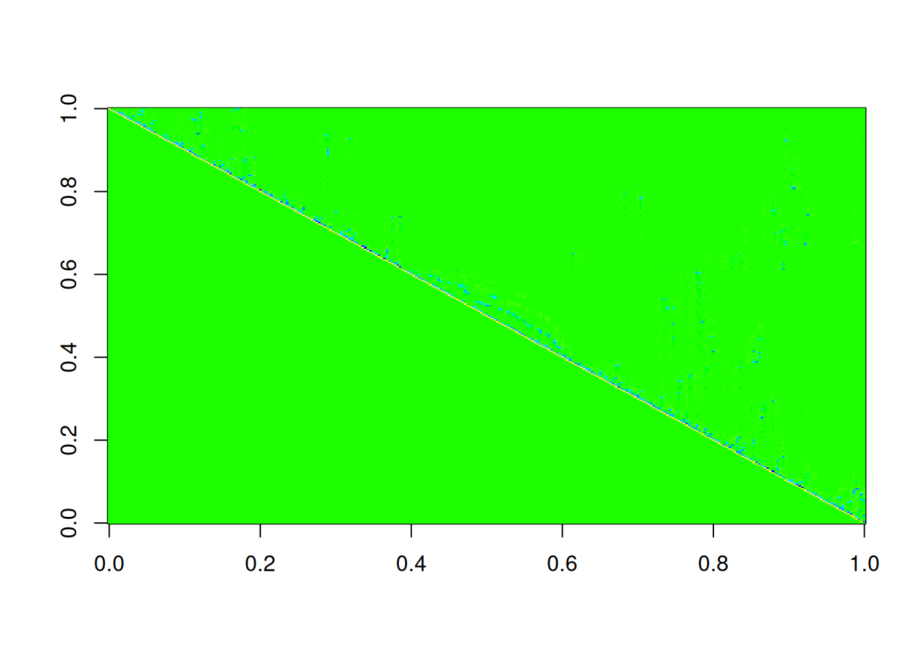
One advantage of SAR models over CAR is that we get a symmetric precision matrix for free. Before we start smoothing, we could generate a sample from this prior in order to check that everything seems to be in order.
This all looks fine, and the fill-in we get for the Cholesky factor doesn’t seem too bad. So now let’s spatially smooth.
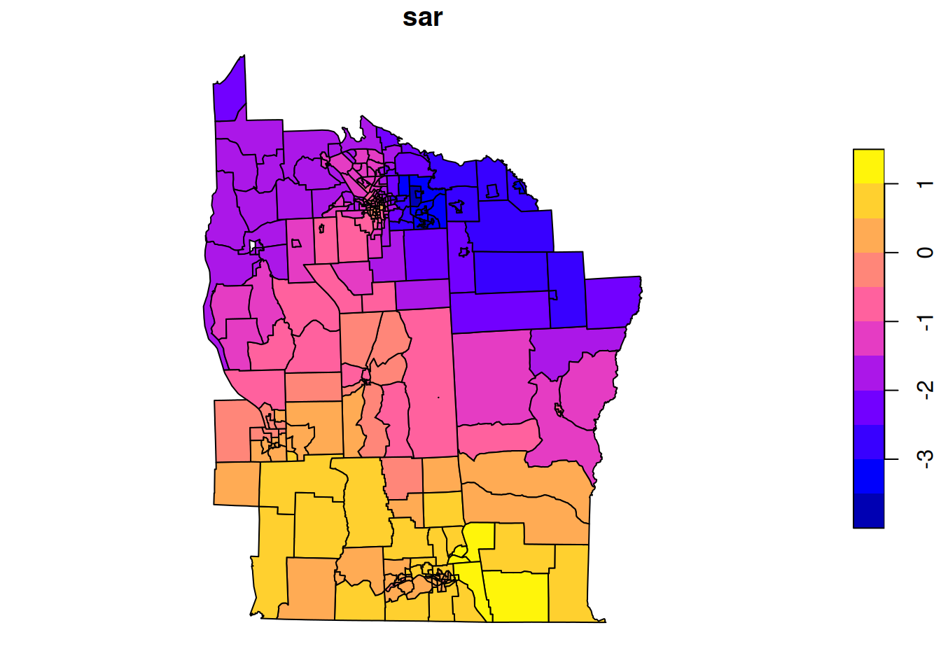
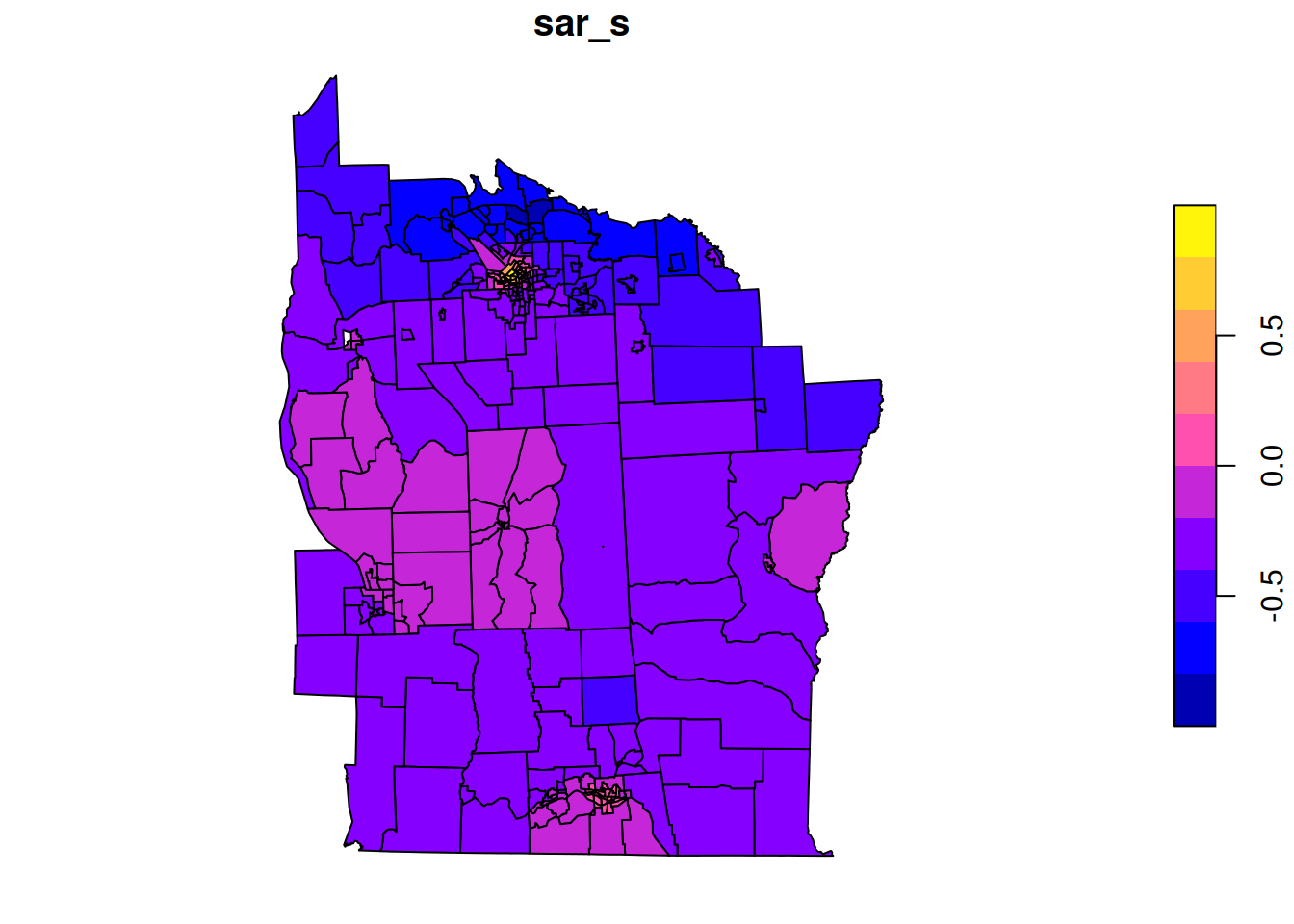
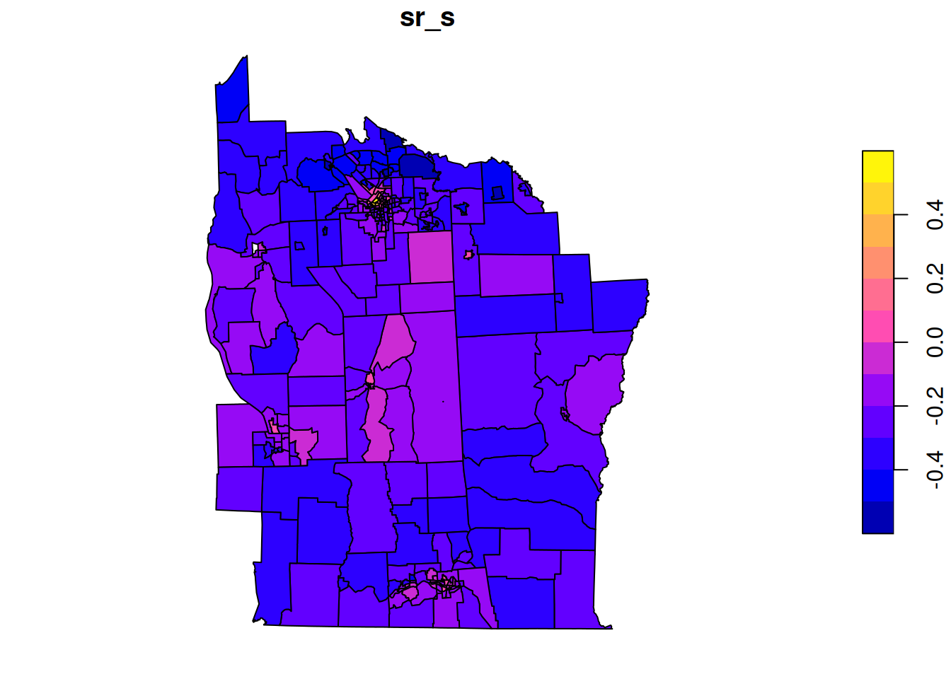
Q_star=Q+diag(n)# obs precision 1 since z scoresb_star=nyd$Z# mean 0 and obs precision 1 since z scoresmu_star=solve(Q_star, b_star)nyd$sar_s=mu_starplot(nyd[,"sar_s"])
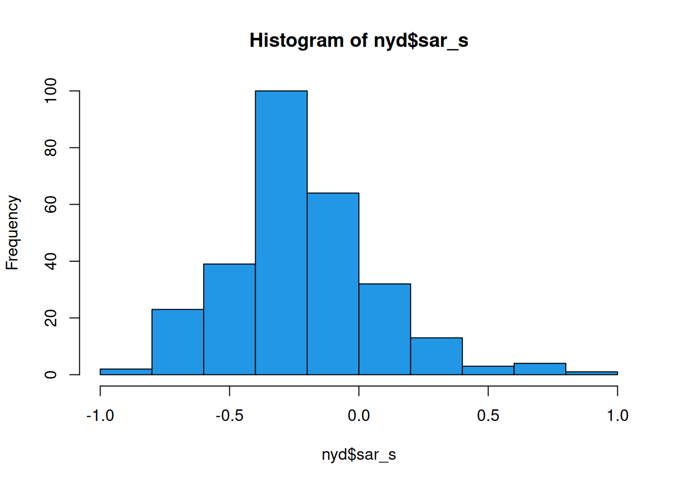
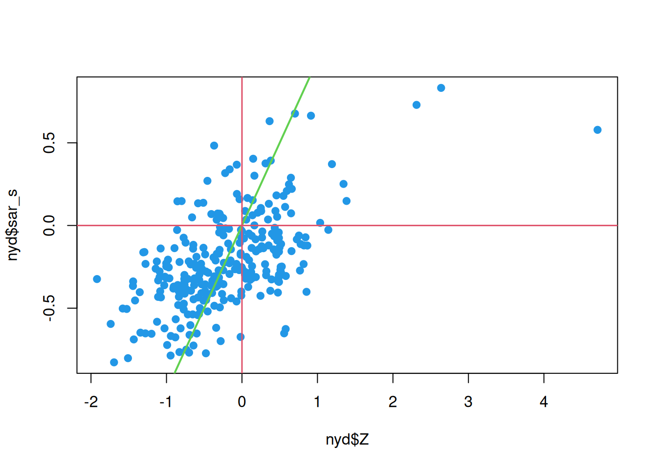
This seems to show a sensible spatial smoothing, suggestive of elevated levels around more densely populated areas, and the histogram of smoothed values indicates that the overall shrinkage has been relatively modest (suggesting that most of the shrinkage has been spatially localised). We can further investigate by comparing smoothed values against raw.
This confirms some overall shrinkage, but that the broad pattern has been preserved.
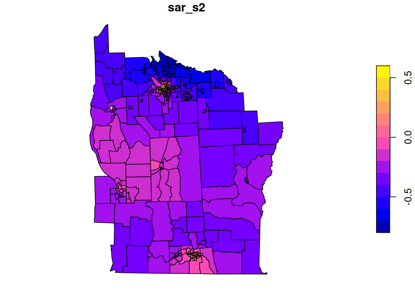
In this analysis we guessed at a residual variance of 0.2, and just assumed a conditional precision of 1 (due to Z being normalised), but neither of these assumptions are necessarily optimal. We could attempt to learn them both from data.
# MVN density, parameterised by mean and precisiondmvnormp=function(x, mu, Q, log=TRUE){Lt=chol(Q)ld=-0.5*length(mu)*log(2*pi)+sum(log(diag(Lt)))-0.5*sum((x-mu)*(Q%*%(x-mu)))if(log)ldelseexp(ld)}# log-likelihood of a conditioned GMRFgmrfll=function(mu, Q, F, Lambda, y){Q_star=Q+t(F)%*%(Lambda%*%F)b_star=Q%*%mu+t(F)%*%(Lambda%*%y)mu_star=solve(Q_star, b_star)dmvnormp(mu, mu, Q)+dmvnormp(y, F%*%mu, Lambda)-dmvnormp(mu, mu_star, Q_star)}Qstd=((diag(n)-t(B))%*%(diag(n)-B))# precision without variance scalingnyd_ll=function(lpar){par=exp(lpar); sigma=par[1]; lambda=par[2]gmrfll(rep(0, n), Qstd/(sigma^2), diag(n), lambda*diag(n), nyd$Z)}nyd_ll(c(0.2, 1))
There are minor differences to the previous smoothing, but the overall picture remains similar.
Task B
Conduct a spatial smoothing using an equally weighted CAR prior rather than SAR. Use maximum likelihood to estimate the CAR conditional variance parameter, \(\kappa\) (kappa), and the observational precision, \(\lambda\) (lambda).
Question 3
Let us now investigate spatial regression for the variable of interest, Z. Let’s start with a simple spatial smoothing (with SAR residuals).
Call: spautolm(formula = Z ~ 1, data = nyd, listw = nb2listw(nyd_nb))

Residuals:
      Min        1Q    Median        3Q       Max
-1.659136 -0.433952 -0.065391  0.434972  4.666104

Coefficients:
             Estimate Std. Error z value Pr(>|z|)
(Intercept) -0.206410   0.066981 -3.0816 0.002059

Lambda: 0.38776 LR test value: 22.793 p-value: 1.8042e-06
Numerical Hessian standard error of lambda: 0.076231

Log likelihood: -297.4879
ML residual variance (sigma squared): 0.47256, (sigma: 0.68743)
Number of observations: 281
Number of parameters estimated: 3
AIC: 600.98
Identify an appropriate spatial regression model for this data. The potentially interesting and useful covariates are PCTOWNHOME, PCTAGE65P, and PEXPOSURE. See ?nydata for (slightly) further details. When you identify a model that you are happy with, plot both the fitted values and the residuals in their spatial context. What does it all mean?
Question 4 (for keen beans)
Task D
Re-do the CAR-based spatial smoothing from Task B, but using sparse matrices and sparse matrix operations from the Matrix package. Use the estimated variance parameters that you have already obtained.