16 Inference for lattice models
16.1 Smoothing lattice data
One of the primary aims of the analysis of areal data and other data on spatial lattices is to smooth noisy observations of an underlying spatial process. This is the spatial analogue of the smoothing of time series using state space models. Here we don’t have a simple sequential structure that will allow us to develop recursive algorithms like the Kalman filter, but we will exploit the sparsity of the model’s conditional independence structure in other ways.
In the previous chapter we have developed models for data on lattices with spatial dependence, so that nearby sites are more highly correlated than distant sites. Much of our attention focused on GMRFs, and so those will form our starting point for thinking about inference. To keep things general, we will assume that we have a GMRF defined on a lattice of \(n\) nodes, of the form \[ \mathbf{X} \sim \mathcal{N}(\pmb{\mu}, \mathsf{Q}^{-1}). \] The mean, \(\pmb{\mu}\), will often be \(\mathbf{0}\). The precision matrix, \(\mathsf{Q}\), is assumed to be sparse, reflecting the conditional independence structure of the graphical model. However, it could arise from either a CAR or SAR model specification, or any other process leading to a sparse precision matrix. \(\mathbf{X}\) is assumed to be a hidden or unobserved process, and we wish to make inferences about it on the basis of some noisy observation process. To begin with we will assume a Gaussian observation model, since that will lead to tractable inference. But again, to keep things reasonably general, we will assume a model for our observed data \(\mathbf{Y}\) of the form \[ (\mathbf{Y}|\mathbf{X}=\mathbf{x}) \sim \mathcal{N}(\mathsf{F}\mathbf{x}, \mathsf{\Lambda}^{-1}). \] The conditional precision matrix, \(\mathsf{\Lambda}\), and the observation matrix, \(\mathsf{F}\), will often be diagonal, with observations corresponding to individual lattice nodes, but this model allows more flexibility. Crucially, our only strict condition is that both \(\mathsf{\Lambda}\) and \(\mathsf{F}\) are sparse. It will be a requirement of our analysis that we do not need to explicitly construct any large dense matrices.
Together, our specification for the “prior” hidden process and the observation model determine a joint model over both \(\mathbf{X}\) and \(\mathbf{Y}\). When we observe data \(\mathbf{Y}=\mathbf{y}\), we will be interested in the “posterior” distribution \(\mathbf{X}|\mathbf{Y}=\mathbf{y}\). For example, the mean of this distribution could be used as our “smoothing” of the data, and samples from it could be used to understand our uncertainty. Since everything in this problem is linear and Gaussian, we could use standard multivariate normal conditioning results in order to compute this distribution. However, given our specification in terms of sparse precision matrices, we can better maintain sparsity by directly computing and recognising the relevant density, as a function of \(\mathbf{x}\). \[\begin{align*} \pi(\mathbf{x}|\mathbf{y}) &\propto \pi(\mathbf{x})\pi(\mathbf{y}|\mathbf{x}) \\ &= \mathcal{N}(\mathbf{x};\pmb{\mu}, \mathsf{Q}^{-1})\mathcal{N}(\mathbf{y};\mathsf{F}\mathbf{x}, \mathsf{\Lambda}^{-1}) \\ &\propto \exp\left\{-\frac{1}{2}(\mathbf{x}-\pmb{\mu})^\top\mathsf{Q}(\mathbf{x}-\pmb{\mu})\right\} \exp\left\{-\frac{1}{2}(\mathbf{y}-\mathsf{F}\mathbf{x})^\top\mathsf{\Lambda}(\mathbf{y}-\mathsf{F}\mathbf{x})\right\} \\ &\propto \exp\left\{-\frac{1}{2}\left[ \mathbf{x}^\top(\mathsf{Q}+\mathsf{F}^\top\mathsf{\Lambda}\mathsf{F})\mathbf{x} - 2\mathbf{x}^\top(\mathsf{Q}\pmb{\mu}+\mathsf{F}^\top\mathsf{\Lambda}\mathbf{y}) \right]\right\}. \end{align*}\] At this point we can observe that this density involves only sparse matrices and sparse matrix operations. By completing the square we recognise it as \[ (\mathbf{X}|\mathbf{Y}=\mathbf{y}) \sim \mathcal{N}\left([\mathsf{Q}+\mathsf{F}^\top\mathsf{\Lambda}\mathsf{F}]^{-1}[\mathsf{Q}\pmb{\mu}+\mathsf{F}^\top\mathsf{\Lambda}\mathbf{y}], [\mathsf{Q}+\mathsf{F}^\top\mathsf{\Lambda}\mathsf{F}]^{-1}\right). \] We note that this Gaussian distribution has a sparse precision matrix, \(\mathsf{Q}^\star = \mathsf{Q}+\mathsf{F}^\top\mathsf{\Lambda}\mathsf{F}\), and that its mean, \(\pmb{\mu}^\star\), can be computed efficiently by computing \(\mathsf{Q}^\star\) and \(\mathbf{b}^\star=\mathsf{Q}\pmb{\mu}+\mathsf{F}^\top\mathsf{\Lambda}\mathbf{y}\), and then solving the sparse linear system \[ \mathsf{Q}^\star \pmb{\mu}^\star = \mathbf{b}^\star \] for \(\pmb{\mu}^\star\). This could be done, for example, using a sparse Cholesky decomposition and sparse forward and backward substitution algorithms. As previously discussed, the posterior mean, \(\pmb{\mu}^\star\), can be used as a spatial smoothing of the data. To explore our uncertainty, we have already seen in Section 15.3.5.2 how to generate exact samples from Gaussians with sparse precision matrices in an efficient manner.
We also know that for parameter inference (and other reasons), it will be useful to be able to compute the marginal likelihood of the data, \(\pi(\mathbf{y})\), in an efficient way. From elementary normal theory we know that the marginal distribution of \(\mathbf{Y}\) is \[ \mathbf{Y} \sim \mathcal{N}(\mathsf{F}\pmb{\mu}, \mathsf{F}\mathsf{Q}^{-1}\mathsf{F}^\top+ \mathsf{\Lambda}^{-1}), \] and that this therefore implies the relevant normal density. Unfortunately, this result is not so useful to us, since the precision matrix of this distribution is not sparse (and clearly, neither is the variance matrix), so it does not give us a convenient way to evaluate the marginal density using only sparse matrix operations. To make further progress, we can use a simple rearrangement of Bayes theorem, often known as Chib’s basic marginal likelihood identity (BMI), \[ \pi(\mathbf{y}) = \frac{\pi(\mathbf{x})\pi(\mathbf{y}|\mathbf{x})}{\pi(\mathbf{x}|\mathbf{y})}. \] Substituting in for our densities we have \[ \pi(\mathbf{y}) = \frac{\mathcal{N}(\mathbf{x};\pmb{\mu},\mathsf{Q}^{-1})\mathcal{N}(\mathbf{y};\mathsf{F}\mathbf{x},\mathsf{\Lambda}^{-1})}{\mathcal{N}(\mathbf{x};\pmb{\mu}^\star,{\mathsf{Q}^\star}^{-1})}, \] and since each term involves a sparse precision matrix, we can think about how to evaluate them efficiently. Of course, in practice, we will evaluate the log of the marginal likelihood, \[ \log\pi(\mathbf{y}) = \log\mathcal{N}(\mathbf{x};\pmb{\mu},\mathsf{Q}^{-1}) + \log\mathcal{N}(\mathbf{y};\mathsf{F}\mathbf{x},\mathsf{\Lambda}^{-1}) - \log\mathcal{N}(\mathbf{x};\pmb{\mu}^\star,{\mathsf{Q}^\star}^{-1}) . \] Note that since the LHS is independent of \(\mathbf{x}\), the RHS must also be, and so we are free to choose any convenient \(\mathbf{x}\) at which to evaluate. Choosing \(\mathbf{x}=\pmb{\mu}\) is often convenient. We now need to think about how to efficiently evaluate the log-density of a multivariate normal with a sparse precision matrix. We will illustrate using the prior term, \(\log\pi(\mathbf{x})\), but exactly the same approach works for the other two terms. Now, \[ \log\mathcal{N}(\mathbf{x};\pmb{\mu},\mathsf{Q}^{-1}) = -\frac{p}{2}\log 2\pi + \frac{1}{2}\log |\mathsf{Q}| - \frac{1}{2}(\mathbf{x}-\pmb{\mu})^\top\mathsf{Q}(\mathbf{x}-\pmb{\mu}), \] and the final quadratic form term clearly requires only sparse matrix-vector multiplication, so the only potential issue is the central determinant term. However, if we have the sparse Cholesky decomposition, \(\mathsf{Q}=\mathsf{L}\mathsf{L}^\top\), then \[ \frac{1}{2}\log |\mathsf{Q}| = \frac{1}{2}\log |\mathsf{L}\mathsf{L}^\top| = \log|\mathsf{L}| = \log\prod_i l_{ii} = \sum_i\log l_{ii}, \] since the determinant of a triangular matrix is simply the product of its diagonal elements, and we are done. A simple illustrative implementation for dense matrices is given below.
Given this function, we can write a function to evaluate the marginal likelihood of a conditioned GMRF as
We will use these functions later.
16.1.1 Areal data
We will illustrate some basic spatial smoothing using the infamous Boston housing dataset, spData::boston. We begin by loading the data.
We can create a neighbour list and plot it as follows.
boston_nb <- spdep::poly2nb(boston.tr)
plot(st_geometry(boston.tr), border="grey")
plot(boston_nb, sf::st_geometry(boston.tr),
    pch=19, cex=0.5, add=TRUE, col="blue")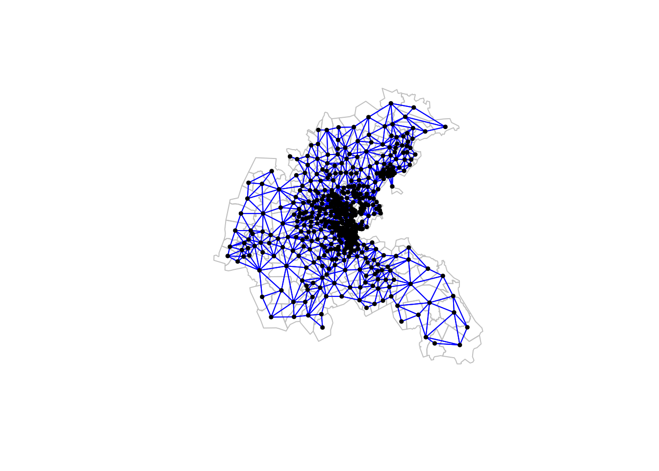
dim(boston.tr)[1] 506 37There are 506 nodes in this graph, each corresponding to a census tract in the Boston metropolitan area. This graph is still of a size that we can do some analysis without the need for sparse matrix libraries, although it is sufficiently large that computationally intensive procedures would benefit from them.
We will illustrate spatial smoothing using some basic house-price data.
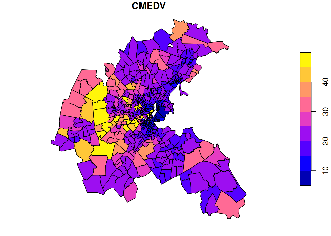
The data is median house price (in thousands of USD) for each area. The plot shows large variations in house prices from area to area, with some overall patterns, but interrupted by adjacent areas with high and low prices, respectively. We might think that house prices will tend to spatially equilibriate over time, so we might prefer to spatially smooth the data to get a better feel for which larger parts of the metropolitan area tend to have higher and lower prices, respectively.
We see that, very roughly, the mean is around 20 and the standard deviation is around 2 (it is very old data!). We can take the mean of the hidden CAR process to be 20. We could also take the conditional variance of the observations to be 4 (so a conditional precision of \(\lambda=1/4\)), and this should help to encourage strong smoothing. Thinking about the specification of the CAR prior itself, we might think that an area with 4 neighbours could vary from the average of those neighbours with a standard deviation of 1/2, and so a variance of 1/4. This suggests choosing \(\kappa=1\) (so that \(\kappa_i=1/4\)). We will see later how we can try to learn about some of these parameters from data, but this should get us started.
We can compute the prior and posterior mean vector and precision matrices, and use the posterior mean as our spatial smoothing, as follows.
mu = 20
kappa = 1
lam = 1/4 # conditional precision of observations
rho = 0.999 # dependence parameter
A = adjW*rho # weight matrix
Kv = kappa / num # kappa vector
Q = (diag(n) - A)/Kv
Q_star = Q + lam*diag(n) # F is the identity here
b_star = Q %*% rep(mu, n) + rep(lam, n)*boston.tr$CMEDV
mu_star = solve(Q_star, b_star) # posterior mean
boston.tr["cmedvs"] = mu_star
plot(boston.tr["cmedvs"], main="Spatial smoothing of house value")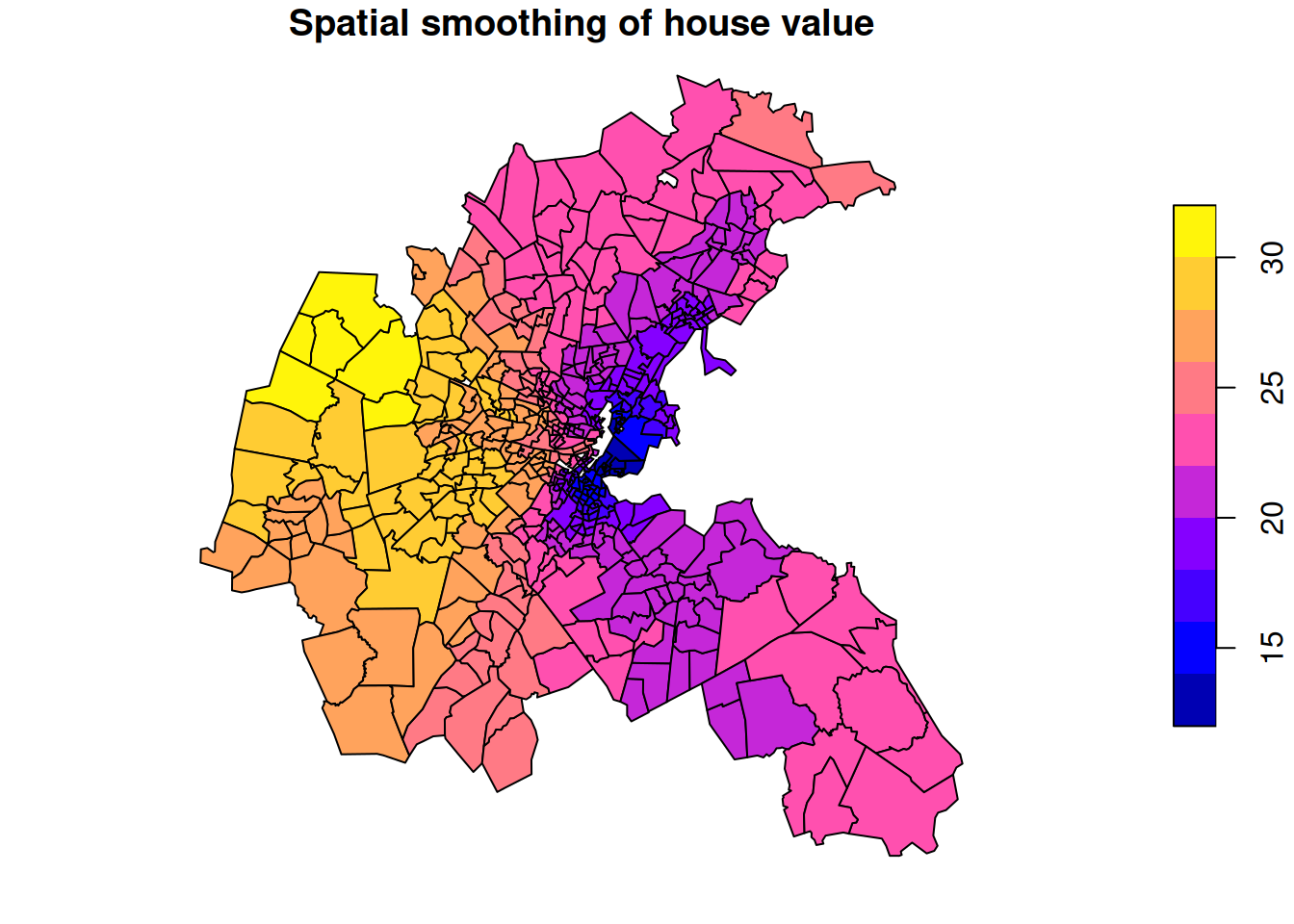
This spatially smoothed data better reveals that the higher value houses tend to be in the west, and that prices are generally lower in the east, with a strong concentration of lower value housing in the harbour area.
16.1.2 Missing data imputation (interpolation on the graph)
Inclusion of the sparse observation matrix, \(\mathsf{F}\), in our model, gives us a lot of flexibility regarding non-standard observation processes. For example, if we had observations that are actually aggregations over multiple nodes, we can accommodate this. Further, we can accommodate missing data very easily by starting from a diagonal \(\mathsf{F}\) and then deleting the rows corresponding to the missing observations. So if we start from an \(n\times n\) diagonal matrix and delete the rows corresponding to \(m\) missing observations, we are left with a \((n-m)\times n\) sparse \(\mathsf{F}\) matrix to map our hidden process onto our actual observed values.
We will illustrate this idea with a very extreme (and artificial) example where we have just three observations. So our sparse \(\mathsf{F}\) matrix will be \(3\times n\), with the 1 in each row corresponding to the location of that observation. We will condition on a very high observation in the west, a very low value in the north, and a medium value in the south.
west = which.min(boston.tr$LON) # index of western most tract
north = which.max(boston.tr$LAT) # northern most tract
south = which.min(boston.tr$LAT) # southern most tract
F = matrix(0, nrow=3, ncol=n)
F[1, west] = 1 # first obs in Western most tract
F[2, north] = 1 # second obs in Northern most tract
F[3, south] = 1 # third obs in Southern most tract
y = c(10, -10, 0) # high obs in west, low obs in north and mid in south
Q_star = Q + t(F) %*% F # assume identity error matrix
b_star = t(F) %*% y # assume mean zero prior
mu_star = solve(Q_star, b_star) # posterior mean
boston.tr["mdi"] = mu_star
plot(boston.tr["mdi"],
main="Missing data imputation (for 3 observations)")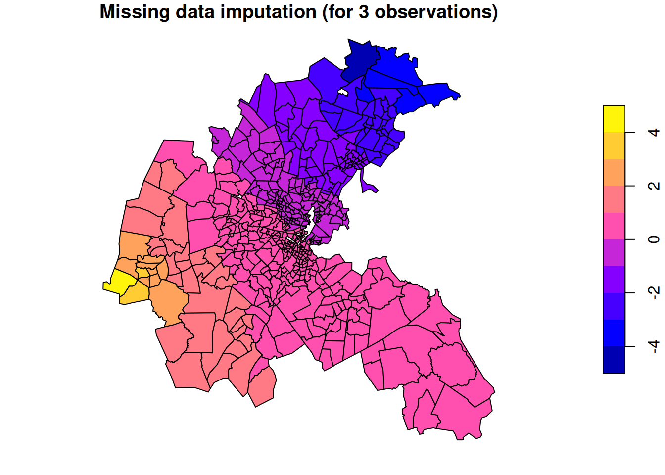
This gives us a nice smooth estimate for the value of the hidden field at each spatial location. It is very much analogous to the Kriging approach to smooth interpolation that we used in the context of continuously varying processes. However, we are only interpolating to nodes of the graph. There is no direct way to interpolate between nodes of the graph, and in the context of areal data, this isn’t really a meaningful thing to contemplate.
The posterior mean gives us a very smoothly varying graph interpolation. But it is just a point estimate at each location, despite the fact that there will often be considerable uncertainty about the actual value of the hidden field. Drawing exact realisations from the posterior process can give us insight into this variability. In the context of missing data imputation, we might want to make several draws, and average over them in some way for a multiple imputation approach. Draws are also often useful in the context of MCMC algorithms for parameter estimation.
Lt_star = chol(Q_star)
set.seed(35)
z = backsolve(Lt_star, rnorm(n))
boston.tr["mds"] = mu_star + z
plot(boston.tr["mds"],
main="Realisation of the posterior hidden process")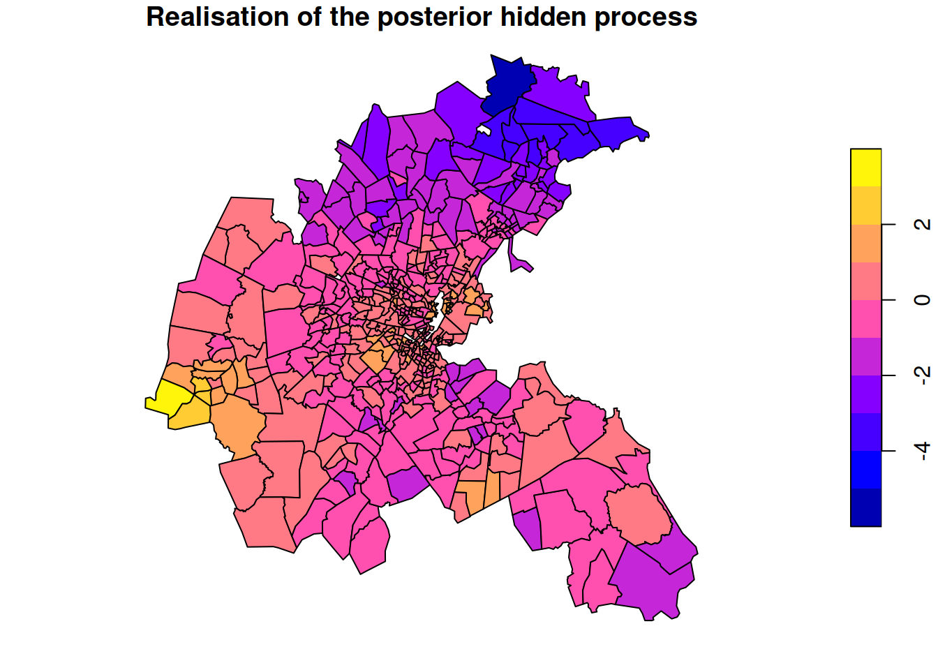
We see that the draw from the posterior looks more “realistic” than the posterior mean, and includes variability from site to site whilst maintaining the overall trends.
16.1.3 Images
Since images are just data on a regular square lattice, we can use the same techniques for smoothing noisy images. This approach works well when the underlying model assumptions are reasonable. So here, that is that the “true” image is quite smooth, and that the noise at each in the observed image is Gaussian and conditionally independent given the true image. All of these assumptions can be problematic in practice. In particular, in many cases the observational noise is spatially correlated, and this matters.
In the case of a smooth underlying image, spectral methods can often be better for image smoothing. Just apply the 2d FFT to the image, keep only the low frequency terms, zero out the rest, and then inverse FFT back to image space. This generally works well for smooth images, and is not affected by observational noise that is correlated over short spatial scales. In practice, people often use the (very closely related) 2d DCT for this purpose.
For images with sharp edges, these simple techniques don’t work so well. If the goal is really image segmentation, see Section 16.4.
16.1.4 Count data
Our previous example of spatial smoothing was the median house price in Boston census tracts. Median house price is a good variable to consider for modelling over a discrete space, as it makes sense to directly compare it between tracts of different sizes or populations. Variables like this are sometimes referred to as intensive or localised, because they represent some kind of intensity that makes sense to to think about existing everywhere in space, and hence can be regarded as a field. Contrast this with the total value of all property inside a tract. This is an example of an extensive variable, some kind of sum, count or aggregate over the region. Many spatial variables are of this form, but they are typically not suitable for direct modelling or comparison across sites, since they depend strongly on some kind of measure of the size of the region, such as its geographic area or its population size. For the example of total property value, we would expect the variable to be much bigger in areas with many properties, even if the value of those properties are similar to those in regions with fewer properties. Extensive variables can often be transformed into intensive variables, and the process of doing this is sometimes referred to as normalisation. Count data, such as the number of events of a particular type that occur in a region, are an example of an extensive variable. If the counts are large, it is typically straightforward to normalise the count into some kind of rate, and then proceed with modelling the underlying rate. But if the counts are small, other issues also arise.
We will explore the issues associated with (small) count data in the context of the NC SIDS dataset. We begin by loading the data.
nc <- st_read(system.file("shapes/sids.gpkg", package="spData")[1])
ncCR85_nb <- read.gal(
system.file("weights/ncCR85.gal",
package="spData")[1],
region.id=as.character(nc$FIPS))We will consider the spatial variable SID79, representing a count of the number of SIDS events in each county in a given time window.
plot(nc["SID79"])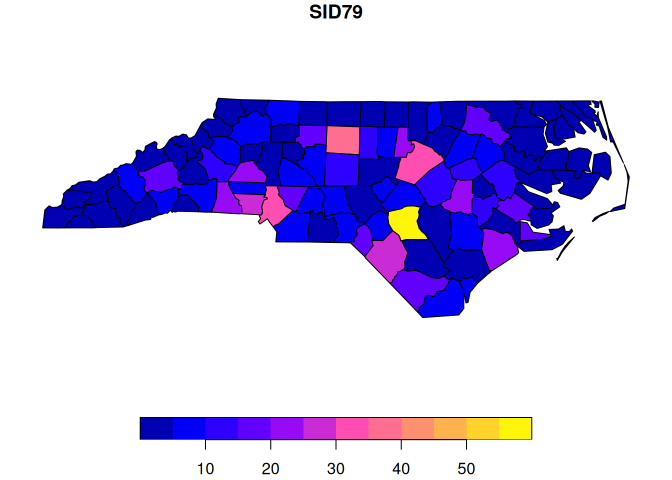
Looking at the plot, we see a bright yellow county. Is this something to worry about? Before getting too concerned, we should bear in mind that these are raw counts, and different counties have very different populations, and hence very different numbers of births. Fortunately, the dataset also contains the number of registered births in the same time window. So we can also look at these.
plot(nc["BIR79"])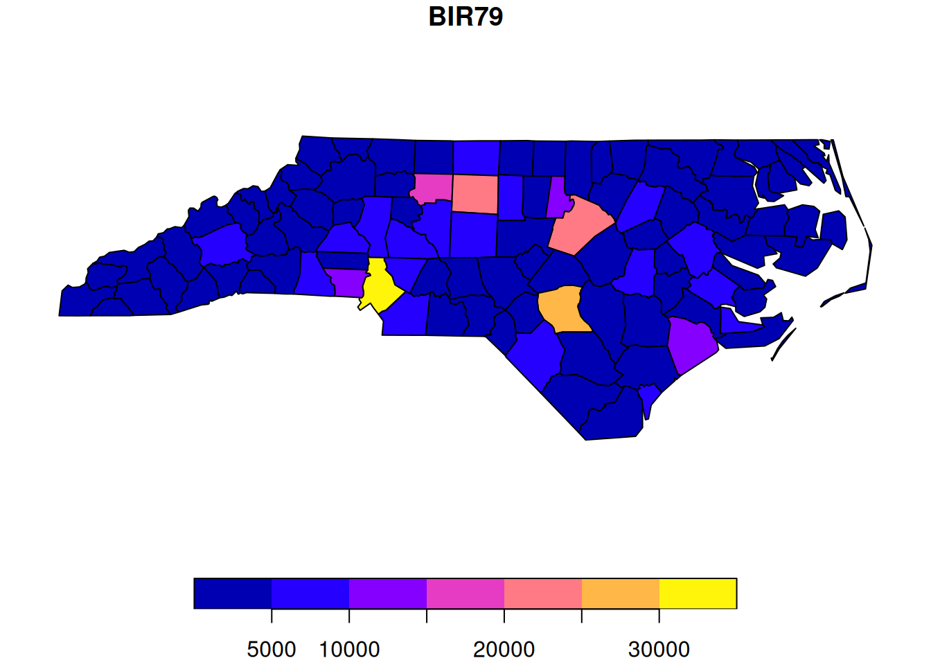
Unsurprisingly, we now see that the counties with the high numbers of SIDS events are also the counties with high numbers of births (presumably due to a larger resident population). We can do a scatter-plot of SIDS against births to confirm.
plot(nc$BIR79, nc$SID79, pch=19, col=4,
main="SIDS against births")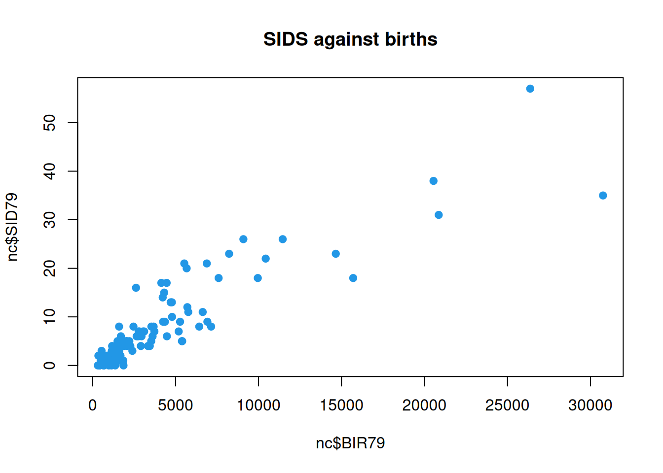
It is clear that the relevant issue is not the raw event count, but the intensity of SIDS events per birth - essentially, the probability that a given birth will lead to a SIDS event. We can begin to explore this by looking at the ratio of SIDS events to births. This process of creating the ratio is an example of normalising the extensive count variable into an intensive rate.
rate = nc$SID79/nc$BIR79
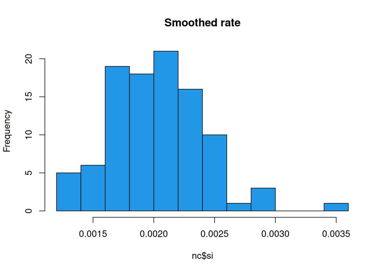
hist(rate, col=4)
The centre of this distribution is at around 0.002 - around 1 in 500 births. But we can also see that some counties have an incidence rate much higher than this. Is that a concern? Let’s plot a choropleth of the ratio.
nc["rate"] = rate
plot(nc["rate"])
Should we be concerned about the county coloured bright yellow? We are now working with an intensive rate which makes sense to compare across areas of different sizes, so there’s no problem there. But let’s look at a scatter-plot of the rate against births.
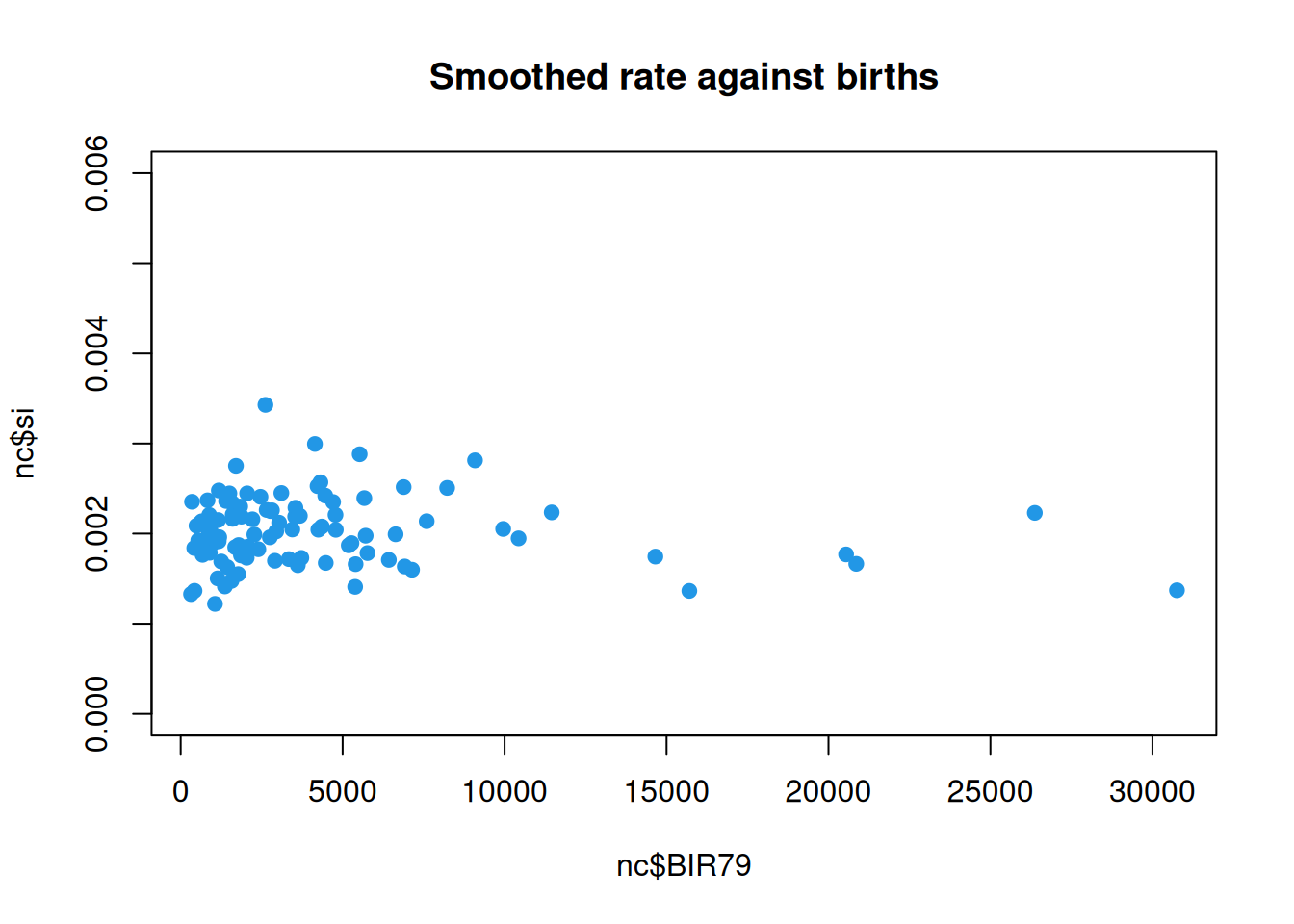
plot(nc$BIR79, rate, pch=19, col=4,
main="Rate against births")
We can immediately see that the counties with the highest ratios are among the smaller counties. But the lowest ratios are also among the smallest counties. Indeed, some smaller counties have zero incidences. None of this should surprise us. The events are random and the variance of the empirical ratio estimate of the intensity decreases as the number of birth events increases. We need a proper statistical model for the data generating mechanism.
We assume that each birth event in county \(i\) has a probability \(p_i\) of leading to a SIDS event. If there are \(m_i\) births (\(m\) for mass or measure), and SIDS events are independent within the county, then the number of SIDS events will be \[ Y_i \sim \text{Bin}(m_i\,, p_i), \] but since the number of births is large and the probability of SIDS is small, it makes sense to instead adopt the model \[ Y_i \sim \text{Po}(m_i p_i). \] So, if we assume some kind of random field model for the \(p_i\), we can condition on the data to obtain a posterior field. But since we don’t have a Gaussian observation model we won’t have a Gaussian posterior. Here, we face a fork in the road. We can either continue to model as accurately as possible, get an intractable posterior, and use MCMC techniques to sample from it, or make approximations to make the problem more tractable.
16.1.5 MCMC approach
We want a spatial model for the intensity field, \(p_i\), but this must be positive, so we can use a log-link. That is, we can adopt a Gaussian CAR model for a field \(X_i\), and then define \(p_i = e^{X_i}\). We then condition on the data to obtain a posterior field. Unfortunately, this posterior field is not Gaussian, so all tractability is lost. Nevertheless, it is straightforward to determine the local characteristics of each node of the posterior hidden field.
The prior local characteristics are \[ X_i|\mathbf{x}_{-i} \sim \mathcal{N}\left(\mu_i+\sum_ja_{ij}(x_j-\mu_j)\, , \kappa_i\right), \] and the observation model is \[ Y_i|x_i \sim \text{Po}(m_ie^{x_i}), \] so the prior local characteristic density is \[ \pi(x_i|\mathbf{x}_{-i}) = \frac{1}{\sqrt{2\pi\kappa_i}}\exp\left\{-\frac{1}{2\kappa_i}\left(x_i-\mu_i-\sum_ja_{ij}(x_j-\mu_j)\right)^2\right\}, \] and the probability mass function of the observation is \[ \pi(y_i|x_i) = \frac{(m_ie^{x_i})^{y_i}}{y_i!}\exp\{-m_ie^{x_i}\}. \] Consequently, the full-conditional for site \(i\) has density \[\begin{align*} \pi(x_i|\mathbf{x}_{-i},y_i) &\propto \pi(x_i|\mathbf{x}_i)\pi(y_i|x_i) \\ &\propto e^{y_ix_i}\exp\left\{-m_ie^{x_i}\right\}\exp\left\{-\frac{1}{2\kappa_i}\left(x_i-\mu_i-\sum_ja_{ij}(x_j-\mu_j)\right)^2\right\}\\ &= \exp\left\{ y_ix_i - m_ie^{x_i} -\frac{1}{2\kappa_i}\left(x_i-\mu_i-\sum_ja_{ij}(x_j-\mu_j)\right)^2 \right\}. \end{align*}\] So, up to a constant, the log full-conditional at site \(i\) is \[ \log\pi(x_i|\cdot) = y_ix_i - m_ie^{x_i} -\frac{1}{2\kappa_i}\left(x_i-\mu_i-\sum_ja_{ij}(x_j-\mu_j)\right)^2 . \] It is a little disconcerting to see an exponential in a log-density, but this is just a feature of Poisson log-link models. So we now know the local characteristics of the posterior random field. It is not analytically tractable, but we can use a component-wise random-walk Metropolis-Hastings to generate samples from it. Furthermore, if there are any unknown parameters in the model, we can put priors on them, and sample from their full-conditionals along with everything else. This gives us a fully Bayesian solution to the problem.
This is in many ways the best approach, but we are trying to avoid MCMC in this course, so we will think about an alternative strategy.
16.1.6 Approximate approach
If we want to maintain some kind of tractability, then we will need to make some approximations of some sort. There are many different ways we could do this, some of which are quite sophisticated and accurate. Here, for simplicity, we will adopt the simplest approach of approximating the Poisson observation model as Gaussian. In this case, we cannot adopt a log-link, since this will destroy the linear Gaussian structure that we need. So we must model the intensity field directly as a CAR and hope that it does not have much mass below zero.
We approximate the SIDS count as \[ Y_i \overset{\cdot}{\sim} \mathcal{N}(m_ip_i, m_ip_i). \] We could work directly with this by using an \(\mathsf{F}\) matrix other than the identity. But it’s slightly easier to work with the empirical rate, \[ Z_i \equiv \frac{Y_i}{m_i} \overset{\cdot}{\sim} \mathcal{N}(p_i, p_i/m_i). \] Unfortunately, our linear Gaussian structure requires that the variance is deterministic. So we can make the further approximation, \[ Z_i\overset{\cdot}{\sim} \mathcal{N}(p_i, \tilde p/m_i), \] where \(\tilde p\) is some fixed overall estimate of \(p\), such as the empirical rate over the whole of NC. Note that if we were doing this seriously, we might consider the use of a variance-stabilizing transformation such as the Anscombe transform or Freeman-Tukey transformation. We will choose \(\tilde p = 0.002\), and we will similarly use this as the mean, \(\mu\), of our CAR prior. The only other thing we need to specify is the \(\kappa\) conditional variance parameter of our CAR prior. Thinking about the distribution of rates across the counties, it seems reasonable to imagine that the conditional standard deviation for a county with 4 neighbours might be 0.0005. This determines \(\kappa=4\times 0.0005^2\). We can compute and plot the smoothed mean as follows.
adj = nb2mat(ncCR85_nb, style="B") # binary adjacency matrix
adjW = nb2mat(ncCR85_nb) # weight matrix with rows summing to one
n = nrow(adj) # number of sites
num = rowSums(adj) # number of neighbours of each site
kappa = 4*0.0005^2 # conditional variance parameter
rho = 0.999 # dependence parameter
mu = 0.002 # mean intensity
lambda_d = nc$BIR79 / mu # diag. of obs. precision mat.
A = adjW*rho # weight matrix
Kv = kappa / num # kappa vector
Q = (diag(n) - A)/Kv # precision matrix
Q_star = Q + diag(lambda_d)
b_star = Q %*% rep(mu, n) + lambda_d*rate
mu_star = solve(Q_star, b_star)
nc["si"] = mu_star # smoothed intensity
plot(nc["si"])
This seems to have worked in the sense that it is qualitatively similar to the raw plot but with differences somewhat smoothed out to reveal larger scale variations. There are still light and dark spots, of course, but it is important to look at the scale. The bright spots on this plot correspond to a much lower estimate than those on the previous plot. Nevertheless, there is one county that is noticeably brighter than the rest. Lets look at a histogram of the smoothed estimates.
So, we see that Scotland, NC does still have a noticeably higher rate than most other counties, but the smoothed rate is now well within a factor of 2 of the bulk of the distribution. If we look at the smoothed rate against births, we see that the pattern is similar to that for the raw rate, and that the rates for the larger counties are essentially unaffected, but that the noisy estimates associated with smaller counties have been shrunk towards the mean level, as we would hope.
Of course, we have made many questionable assumptions along the way, so a great deal of further investigation would be required before drawing any firm conclusions. In particular, we have just guessed at a bunch of variance parameters which may be possible to learn from the data.
16.2 Estimation of model parameters
16.2.1 Gaussian models
For Gaussian observation of a GMRF, we have seen that it is possible to evaluate the marginal model likelihood, \(\pi(\mathbf{y})\), efficiently, using only sparse matrix operations. But both the prior GMRF model and the observation model may contain parameters whose values are uncertain. In this case we can regard the marginal likelihood as conditional on parameters, \(\pmb{\theta}\), and write it \(\pi(\mathbf{y}|\pmb{\theta})\). But this is just the model likelihood, \(L(\pmb{\theta};\mathbf{y})\). We can use this likelihood for inferential purposes, and in particular, can numerically optimise it to estimate parameters.
It is notoriously difficult to estimate the dependence parameter, \(\rho\), from data, so it’s probably best to not even try; see Section 16.3 for some simple empirical methods for assessing spatial dependence. Mean and variance parameters can sometimes be estimated reasonably well, given sufficient informative data, but even then there can be issues with identifiability and confounding. Caution is required.
To illustrate, we will return to the Boston housing data, which has more data and a simpler set up.
adj = nb2mat(boston_nb, style="B") # binary adjacency matrix
adjW = nb2mat(boston_nb) # weight matrix with rows summing to one
n = nrow(adj) # number of sites
num = rowSums(adj) # number of neighbours of each site
rho = 0.999 # CAR dependence parameter
kappa = 1 # CAR conditional variance parameter
A = adjW*rho # weight matrix
Kv = kappa / num
Q = (diag(n) - A)/KvWe will not attempt to learn \(\rho\) or \(\kappa\), as these parameters are problematic. Instead we will learn the CAR mean, \(\mu\) and \(\lambda\), the conditional precision of the observations. We can define a likelihood function and test it out for our previously assumed parameters using the gmrfll function we defined earlier.
bo_ll = function(lpar) {
    par = exp(lpar); mu=par[1]; lam=par[2]
    gmrfll(rep(mu, n), Q, diag(n), lam*diag(n), boston.tr$CMEDV)
}

bo_ll(log(c(20, 0.25)))
[1] -4361.758So, our previous parameter settings of \(\mu=20\), \(\lambda=1/4\) give a log-likelihood of around -4,362. Can we do better? Let’s try feeding this to optim.
$par
[1]  3.115961 -4.335183

$value
[1] -1827.963

$counts
function gradient
      57       NA

$convergence
[1] 0

$message
NULLexp(opt$par)[1] 22.55509472 0.01309948We see that it has found a much better log-likelihood of around -1,828, for parameters \(\mu=22.6\), \(\lambda=0.013\). The mean hasn’t changed much, but this is a significantly smaller precision, corresponding to a larger observational variance. Using these parameters will therefore lead to more smoothing (since the model will pay less attention to the data).
16.2.2 Non-Gaussian models
For models with a GMRF prior but non-Gaussian observation model, things are a little more tricky, since the marginal likelihood \(\pi(\mathbf{y}|\pmb{\theta})\) is intractable. Fortunately, the complete-data likelihood, \(\pi(\mathbf{x},\mathbf{y}|\pmb{\theta})=\pi(\mathbf{x}|\pmb{\theta})\pi(\mathbf{y}|\mathbf{x},\pmb{\theta})\), is tractable. This provides the possibility of using data-augmentation strategies of various sorts. MCMC algorithms which impute the hidden field along with model parameters are very popular. Also, in many simple cases, an approximate method known as INLA works extremely well, and avoids MCMC.
For non-Gaussian prior models, things are even more tricky, since we typically can’t even evaluate the likelihood function. The normalising constant of the likelihood is typically intractable away from the Gaussian case. This is very problematic since it is a function of the model parameters. Bayesians are used to the idea of the normalising constant cancelling out of Metropolis-Hastings ratios, but this happens because that normalising constant is a function of the data, which is fixed. Here, the normalising constant does not cancel out (for parameters in the prior model), so standard MCMC techniques don’t help (parameters in the observation model can be handled with standard MCMC approaches). There are some advanced MCMC techniques which can potentially help (eg. the “exchange algorithm”), but they are not straightforward. In practice, people often replace the likelihood with the pseudo-likelihood, which is just the product of full-conditionals, and optimise that. This can often work surprisingly well for point estimation of parameters.
These techniques are beyond the scope of this course.
16.3 Empirical measures of spatial dependence
It is difficult to do formal statistical inference for the spatial dependence parameters in MRF models, but we can nevertheless try to understand and quantify the degree of spatial dependence apparent in a dataset by using simple empirical measures of spatial association. There are two commonly used measures for data on a lattice. They both require a weight matrix, \(\mathsf{W}\) (with zero diagonal), describing the purported neighbourhood structure. This could be a simple binary adjacency matrix, or could be weighted in the case of weighted edges (like the \(\mathsf{A}\) matrix in a CAR model).
16.3.1 Moran’s I
Moran’s I is the lattice equivalent of a covariogram-style estimate of spatial association, and can be loosely interpreted like a correlation coefficient, with values close to 1 indicating a high degree of spatial association, and values close to zero suggesting little spatial dependence. \[
I = \frac{\displaystyle n\sum_{i,j}w_{ij}(y_i-\bar{y})(y_j-\bar{y})}{\displaystyle \left(\sum_{i,j}w_{ij}\right)\left(\sum_i(y_i-\bar{y})^2\right)}.
\] In R it is available as spdep::moran.test. We can use this for the Boston house price data.
moran.test(boston.tr$CMEDV, nb2listw(boston_nb))
    Moran I test under randomisation

data:  boston.tr$CMEDV
weights: nb2listw(boston_nb)

Moran I statistic standard deviate = 23.558, p-value < 2.2e-16
alternative hypothesis: greater
sample estimates:
Moran I statistic       Expectation          Variance
     0.6322686784     -0.0019801980      0.0007248376
We see this gives a relatively high value, indicating a high degree of spatial dependence. We can see what would happen in the case of little spatial dependence by randomly permuting the observations to deliberately break the spatial association.
moran.test(sample(boston.tr$CMEDV), nb2listw(boston_nb))
    Moran I test under randomisation

data:  sample(boston.tr$CMEDV)
weights: nb2listw(boston_nb)

Moran I statistic standard deviate = -1.1305, p-value = 0.8709
alternative hypothesis: greater
sample estimates:
Moran I statistic       Expectation          Variance
    -0.0324174020     -0.0019801980      0.0007248376
We see this give a low value, as we would expect.
16.3.2 Geary’s C
Geary’s C is the lattice equivalent of a variogram-style estimate of spatial association. Here, low values correspond to high spatial association and values close to one indicate little spatial association. \[
C = \frac{\displaystyle (n-1)\sum_{i,j}w_{ij}(y_i-y_j)^2}{\displaystyle 2\left(\sum_{i,j}w_{ij}\right)\left(\sum_i(y_i-\bar{y})^2\right)}.
\] In R it is available as spdep::geary.test. For the Boston house price data we get
geary.test(boston.tr$CMEDV, nb2listw(boston_nb))
    Geary C test under randomisation

data:  boston.tr$CMEDV
weights: nb2listw(boston_nb)

Geary C statistic standard deviate = 20.383, p-value < 2.2e-16
alternative hypothesis: Expectation greater than statistic
sample estimates:
Geary C statistic       Expectation          Variance
     0.3846079676      1.0000000000      0.0009114881
which is fairly small, indicating a high degree of spatial association. By contrast, if we randomly permute the observations to break the spatial association,
geary.test(sample(boston.tr$CMEDV), nb2listw(boston_nb))
    Geary C test under randomisation

data:  sample(boston.tr$CMEDV)
weights: nb2listw(boston_nb)

Geary C statistic standard deviate = 1.2019, p-value = 0.1147
alternative hypothesis: Expectation greater than statistic
sample estimates:
Geary C statistic       Expectation          Variance
     0.9637125891      1.0000000000      0.0009114881
we get a value close to one, as we would expect.
16.4 Image (and graph) segmentation
Sometimes given an image (or other spatial data on a lattice), it is desired to segment the image into a small number of distinct classes or categories. An example of binary segmentation might be separating “foreground” from “background”. An example for landsat images might be to classify pixels according to land use, as “urban”, “rural” or “water”, etc.
There are many ways one could approach this segmentation task, but one way that fits with the kinds of spatial auto-regressive models that we have been developing, would be to use a Potts model prior. This is analytically intractable, but somewhat amenable to MCMC methods such as the Gibbs sampler. We have seen that the local characteristics of the Potts model are \[ \pi(x_i|\mathbf{x}_{-i}) \propto \exp\left\{\psi\sum_{j:j\sim i}w_{ij}\mathbb{I}(x_i=x_j)\right\}. \] Assuming conditionally independent observations, we can write the (arbitrary) observation model likelihood as \[ f_i(y_i|x_i) = \exp\{h_i(y_i|x_i)\}, \quad\text{where}\quad h_i(y_i|x_i)=\log f_i(y_i|x_i). \] A physicist might refer to the \(h_i(\cdot)\) as an external field. Combining with the local characteristics, this gives full-conditionals for the hidden field of the form \[ \pi(x_i|\mathbf{x}_{-i},\mathbf{y}) \propto \exp\left\{h_i(y_i|x_i) + \psi\sum_{j:j\sim i}w_{ij}\mathbb{I}(x_i=x_j)\right\}. \] We can then normalise these as \[ \pi(x_i|\mathbf{x}_{-i},\mathbf{y}) = \frac{\displaystyle\exp\left\{h_i(y_i|x_i) + \psi\sum_{j:j\sim i}w_{ij}\mathbb{I}(x_i=x_j)\right\}}{\displaystyle\sum_{k=0}^{K-1} \exp\left\{h_i(y_i|k) + \psi\sum_{j:j\sim i}w_{ij}\mathbb{I}(k=x_j)\right\}},\quad x_i\in\{0,1,\ldots,K-1\}, \] or, if we prefer, \[ \mathbb{P}(x_i=k|\mathbf{x}_{-i},\mathbf{y}) = \frac{\displaystyle\exp\left\{h_i(y_i|k) + \psi\sum_{j:j\sim i}w_{ij}\mathbb{I}(k=x_j)\right\}}{\displaystyle\sum_{k'=0}^{K-1} \exp\left\{h_i(y_i|k') + \psi\sum_{j:j\sim i}w_{ij}\mathbb{I}(k'=x_j)\right\}},\quad k\in\{0,1,\ldots,K-1\}. \] These are simple categorical distributions which can be easily sampled as part of a Gibbs sampler. Any unknown parameters in the observation model can also be handled using standard MCMC techniques. Inference for \(\psi\) is difficult, due to the intractable normalising constant of the Potts model.
16.5 Spatial regression modelling
Spatial regression is concerned with regression modelling for spatial data, attempting to properly account for the spatial context. This is a huge topic that we do not have time to explore properly, here. We will focus on the simplest case of linear models with spatially correlated residuals.
16.5.1 Spatial linear models
Here, we have a linear model, \[ \mathbf{Y} = \mathsf{X}\pmb{\beta} + \mathbf{Z}, \] with residuals, \(\mathbf{Z}\) that are not iid, but instead spatially correlated. For example, they could have a SAR or CAR prior. In the case of basic linear regression modelling, SAR residuals are slightly simpler to implement, and this may be one of the reasons for the continued popularity of SAR models. We can define SAR residuals via \[ \mathbf{Z} = (\mathbb{I}-\mathsf{B})^{-1}\pmb{\varepsilon},\quad \pmb{\varepsilon}\sim \mathcal{N}(\mathbf{0},\sigma^2\mathbb{I}), \] and substitute in to our linear model to get \[ (\mathbb{I}-\mathsf{B})(\mathbf{Y}-\mathsf{X}\pmb{\beta}) = \pmb{\varepsilon}. \] But now it is clear that if we define \(\mathbf{Y}'=(\mathbb{I}-\mathsf{B})\mathbf{Y}\) and \(\mathsf{X}'=(\mathbb{I}-\mathsf{B})\mathsf{X}\), then we have the standard linear model, \[ \mathbf{Y}' = \mathsf{X}'\pmb{\beta}+\pmb{\varepsilon}, \] which can be solved in the usual ways.
16.5.2 Example: Boston data
There are R functions to fit models of this form in the spatialreg package.
The function spatialreg::spautolm (spatial-auto-regressive-linear-model) fits linear models as just described. We can use standard R model formula notation, and just need to pass in a weighted neighbour list for the spatial context. Here we look at the effect of crime and pollution on house value in the Boston housing dataset. We can square-root transform the response and log-transform the crime variable to make them more Gaussian.
mod = spautolm(sqrt(CMEDV) ~ log(CRIM) + NOX,
               listw=nb2listw(boston_nb), data=boston.tr)
summary(mod)
Call: spautolm(formula = sqrt(CMEDV) ~ log(CRIM) + NOX, data = boston.tr,
listw = nb2listw(boston_nb))
Residuals:
Min 1Q Median 3Q Max
-1.495556 -0.289532 -0.058344 0.200572 2.407794
Coefficients:
Estimate Std. Error z value Pr(>|z|)
(Intercept) 6.144025 0.403280 15.2351 < 2.2e-16
log(CRIM) -0.135100 0.029436 -4.5895 4.442e-06
NOX -3.054440 0.674516 -4.5283 5.945e-06
Lambda: 0.82333 LR test value: 380.19 p-value: < 2.22e-16
Numerical Hessian standard error of lambda: 0.027824
Log likelihood: -408.7508
ML residual variance (sigma squared): 0.24581, (sigma: 0.49579)
Number of observations: 506
Number of parameters estimated: 5
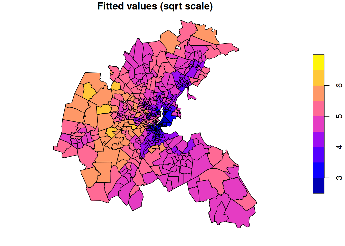
AIC: 827.5All of the usual regression modelling issues apply. We can see that the coefficients for both the crime and pollution variables are negative, suggesting that these are both negatively associated with house value (though as always, the direction of causation may not be clear). Lambda is the estimated spatial dependence parameter (values close to one indicate high spatial dependence). We can plot the fitted values in the usual way.
If we want a pure spatial smoothing model without any covariates, just regress on 1.
Call:
spautolm(formula = sqrt(CMEDV) ~ 1, data = boston.tr, listw = nb2listw(boston_nb))

Residuals:
      Min        1Q    Median        3Q       Max
-1.717387 -0.322622 -0.072255  0.184349  2.394600

Coefficients:
            Estimate Std. Error z value  Pr(>|z|)
(Intercept)   4.5289     0.1545  29.313 < 2.2e-16

Lambda: 0.84728 LR test value: 472.04 p-value: < 2.22e-16
Numerical Hessian standard error of lambda: 0.024269

Log likelihood: -447.3603
ML residual variance (sigma squared): 0.28171, (sigma: 0.53077)
Number of observations: 506
Number of parameters estimated: 3
AIC: 900.72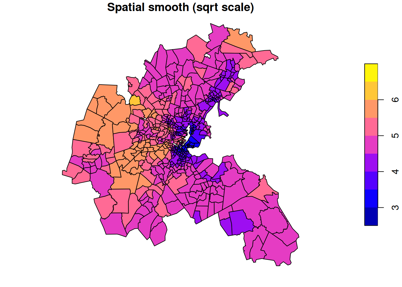
We don’t have to transform the response if we want something more comparable to what we did previously.
Call:
spautolm(formula = CMEDV ~ 1, data = boston.tr, listw = nb2listw(boston_nb))

Residuals:
      Min        1Q    Median        3Q       Max
-16.22689  -3.15296  -0.98131   1.45250  26.14904

Coefficients:
            Estimate Std. Error z value  Pr(>|z|)
(Intercept)  21.4746     1.4015  15.322 < 2.2e-16

Lambda: 0.82033 LR test value: 397.29 p-value: < 2.22e-16
Numerical Hessian standard error of lambda: 0.027178

Log likelihood: -1640.775
ML residual variance (sigma squared): 32.085, (sigma: 5.6644)
Number of observations: 506
Number of parameters estimated: 3
AIC: 3287.6
By default, this function fits SAR residuals. It can also fit CAR models by specifying family="CAR", but in this case you need to ensure that the CAR weights are correctly symmetrised for a consistent specification.
16.5.3 Spatial generalised linear mixed effects models
Of course, there are also R functions and packages for spatial forms of generalised linear models, which are more appropriate for count data, for example. In this case, it is common to introduce the spatial context via random effects having a CAR distribution, and to fit the models via MCMC (or INLA). The details of these models are beyond the scope of this course.