MATH4341: Spatio-temporal statistics

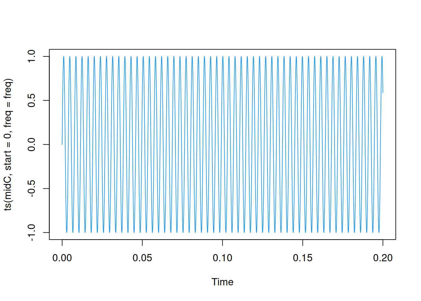
Term 2: Temporal modelling and time series analysis

Computer Lab 3: Spectral methods and digital audio

Load up RStudio via your favourite method. If you can’t use RStudio for some reason, most of what we do in these labs can probably be done using WebR, but the instructions will assume RStudio. You will also want to have the web version of the lecture notes to refer to.

Question 1

Reproduce all of the plots and computations from Chapter 5 of the lecture notes by copying and pasting each code block in turn. Make sure you understand what each block is doing.

Question 2

In the context of the statistical analysis of time series data, we are typically concerned with the spectral analysis of random time series, so that is what we have concentrated on in the lectures. However, for developing intuition about spectral methods (and especially the DFT/FFT), it can be helpful to also look at deterministic time series or signals. Musical notes and related tones and sounds are good examples of signals that are not (very) random but have simple/interesting spectra.

Pure tones

We will start by looking at the simplest possible sound: a pure tone. This is just a sine wave of a given fixed (audible) frequency. The audible range goes from around 20 Hz to 20 kHz, where one Hertz (Hz) is one full sinusoidal oscillation per second. The note “middle C” has a frequency of (roughly) 262 Hz. A natural sound is a signal in continuous time. In digital audio this continuous signal is sampled in discrete time as a time series, typically being recorded at a sampling rate of 44.1kHz (ie. 44,100 times per second), with the amplitude of the signal stored as a floating point number restricted to the range [-1, 1]. So, a wave with an amplitude of 1 will be as loud as possible, whereas a wave with an amplitude of (say) 0.1 will sound much quieter.

Let’s create a time series representing the note “middle C” for a duration of 0.2 seconds. First, we create a vector of times, and then create our signal by applying the sine function with the appropriate frequency.

freq = 44100
times = seq(0, 0.2, by = 1/freq)
midC = sin(2*pi*262*times)
plot(ts(midC, start=0, freq=freq), col=4)

The DFT is all about decomposing a signal into a sum of sinusoidal components. Since this signal is a pure tone, its DFT is especially simple.

length(midC)

[1] 8821

spec = abs(fft(midC))
length(spec)

[1] 8821

plot(ts(spec), col=3)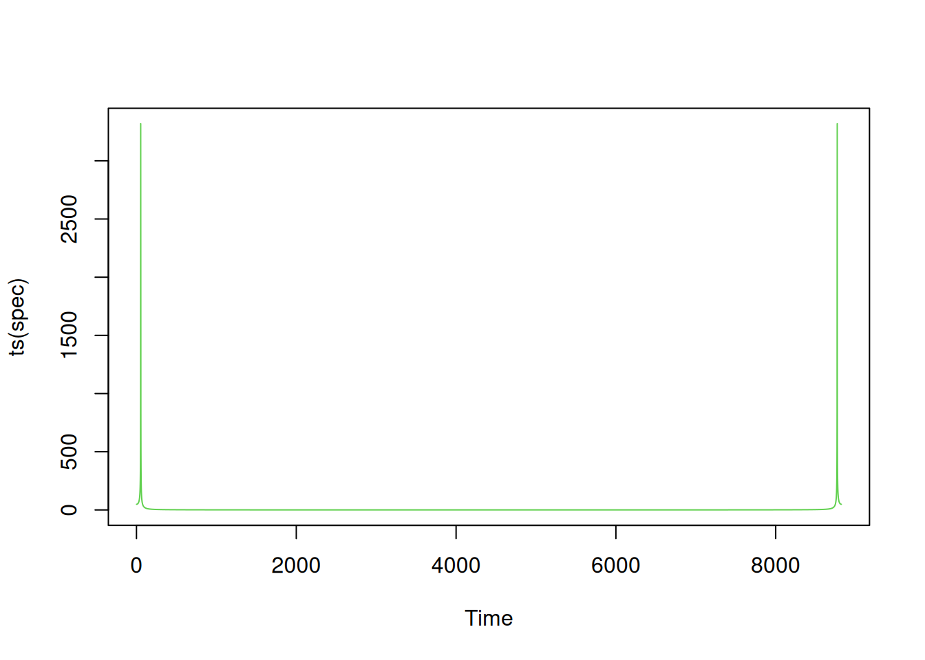

We see that the DFT is essentially zero, but with a strong peak near the two end points. We know that for a real signal, the RHS of the DFT will be just a mirror image of the LHS, so let’s zoom in on the first peak.

plot(ts(spec[1:150]), col=3)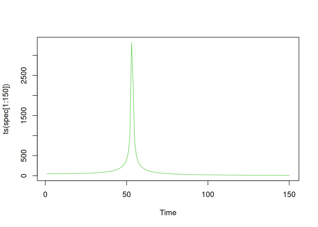

which.max(spec[1:150])

[1] 53

So, we have a single sharp peak at the DFT coefficient with an index (in R) of 53. Since R has 1-based indexing, and the DFT is 0-based, this corresponds to the DFT coefficient numbered 52. Since the DFT has been applied to a time series of length 8821, this corresponds to a frequency, in time series time steps, of

52 / 8821

[1] 0.005895023

but since the time series itself has a frequency of 44.1 kHz, this corresponds to a frequency, in Hz, of

44100 * 52 / 8821

[1] 259.9705

# or
freq * 52 / length(spec)

[1] 259.9705

ie. a frequency close to 260 Hz, which is what we would expect. Note that due to the discrete sampling, the DFT doesn’t give us back the exact frequency we started with, but something very close, since the exact frequency of 262 was not one of the DFT frequencies. This is also why the DFT coefficients nearby the peak are not exactly zero.

Broadly speaking, the DFT shows us the frequencies present in a signal. In particular, it allows us to determine the (approximate) frequency of any pure tones present from the corresponding peaks in the spectrum.

The sound package in R

There is a CRAN package for working with sound samples in R, called sound. Once it is installed (install.packages("sound")), it can be loaded and used in the usual way.

library(sound)
help(package="sound")

We can turn our time series representation of a sound into a sound sample object with

midCsamp = as.Sample(midC)
midCsamp

type      : mono
rate      : 44100 samples / second
quality   : 16 bits / sample
length    : 8821 samples
R memory  : 35284 bytes
HD memory : 17686 bytes
duration  : 0.2 seconds

str(midCsamp)

List of 3
 $ sound: num [1, 1:8821] 0 0.0373 0.0746 0.1118 0.1488 ...
 $ rate : num 44100
 $ bits : num 16
 - attr(*, "class")= chr "Sample"

The raw data can be extracted from a sample object either by using the sound function, or by accessing the $sound attribute. If you have appropriate hardware and have it configured correctly, you may be able to play a sample using your speakers

play(midCsamp)

Don’t worry if this doesn’t work for you in the computer practical - it is not essential to the tasks. Regardless, you can save a sound sample as a WAV file with

saveSample(midCsamp, "midC.wav", overwrite=TRUE)

which you should then be able to play with more-or-less any digital audio software. Obviously, there is a corresponding loadSample function which reads in a WAV file and returns a sample object.

There are several other functions in the package for synthesising and manipulating sound samples. For example, we could have more easily generated our pure tone with

midCs = Sine(262, 0.2)
# play(midCs)

and can synthesise two pure notes separated by a gap with

tune = appendSample(Sine(262, 0.2), Silence(0.1, rate=freq), 
  Sine(440, 0.3))
tune

type      : mono
rate      : 44100 samples / second
quality   : 16 bits / sample
length    : 26460 samples
R memory  : 105840 bytes
HD memory : 52964 bytes
duration  : 0.6 seconds

plot(tune)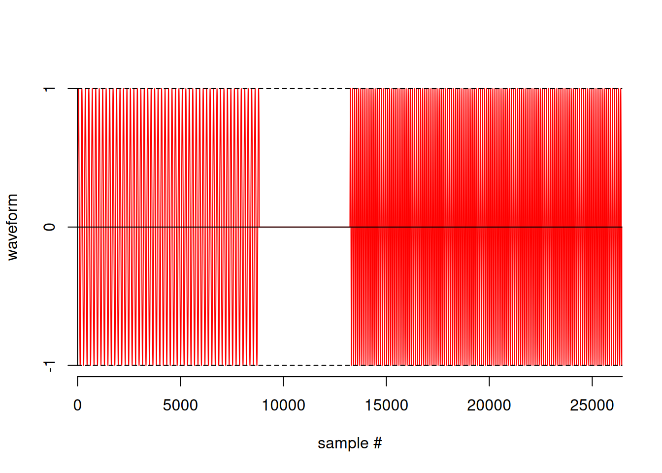

## or
plot(ts(sound(tune)[1,], start=0, freq=freq), col=4)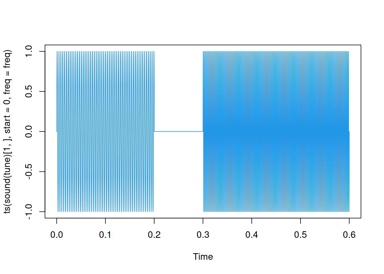

# play(tune)

If we understand something about musical notes, we can start to synthesise more interesting tunes.

semitone = function(h, base = 440)
  base * 2^(h/12)

tune = appendSample(
    Sine(semitone(10), 0.2), Silence(0.1, rate=1440),
    Sine(semitone(12), 0.2), Silence(0.1, rate=1440),
    Sine(semitone(8), 0.2), Silence(0.1, rate=1440),
    Sine(semitone(-4), 0.2), Silence(0.1, rate=1440),
    Sine(semitone(3), 0.4)
    )

# play(tune)

Unfortunately, we don’t have time to explore music theory now.

Touch-tone phones

A traditional land-line telephone requests a number to be connected to by sending an associated sequence of tones. The system used is known as dual-tone multi-frequency (DTMF) signalling. Each number on the phone keypad sends a tone that is made up of two pure tones - one corresponding to the keypad row, and one corresponding to the keypad column. The keypad frequencies for the four rows are: 697, 770, 852 and 941 Hz, and for the three columns are 1209, 1336 and 1477 Hz. It is useful to note that all of the row frequencies are below 1kHz and all of the column frequencies are above 1kHz, and we will make use of this fact later.

Since the number “1” is in the first row and first column of the keypad, the dual-tone that is played will consist of sine waves of frequencies 697 and 1209 superimposed (added). We can generate this using the sound package with

one = 0.5*(Sine(697, 0.2) + Sine(1209, 0.2))
plot(one)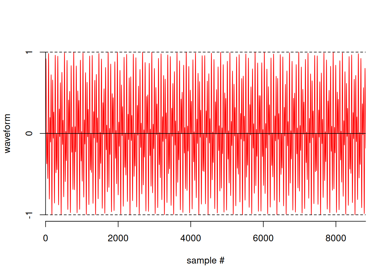

plot(one[1:1000])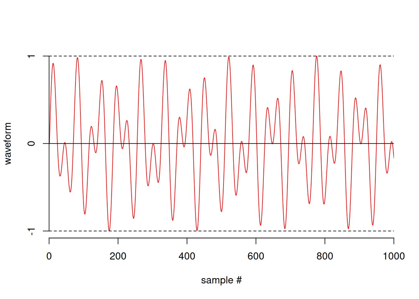

# play(one)

Note the factor of 0.5 in order to ensure that our sample doesn’t get “clipped” due to failing to stay within the range [-1, 1]. This dual-tone is made from two sine waves, and we should be able to see that by looking at the DFT of the sample.

data = sound(one)[1,]
spec = abs(fft(data))
plot(ts(spec), col=3)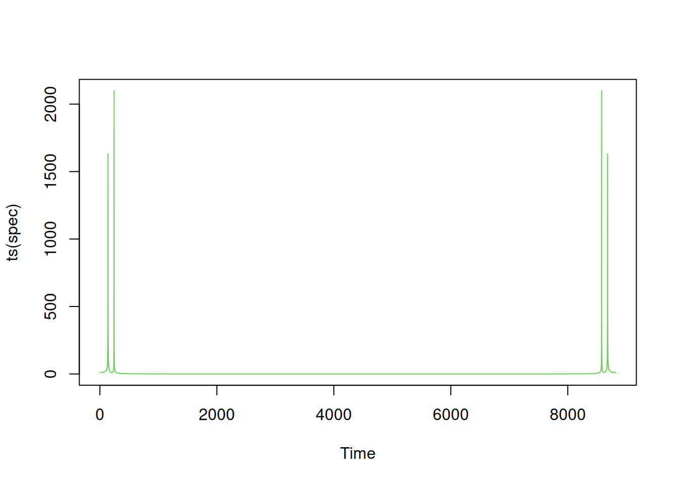

plot(ts(spec[1:500]), col=3)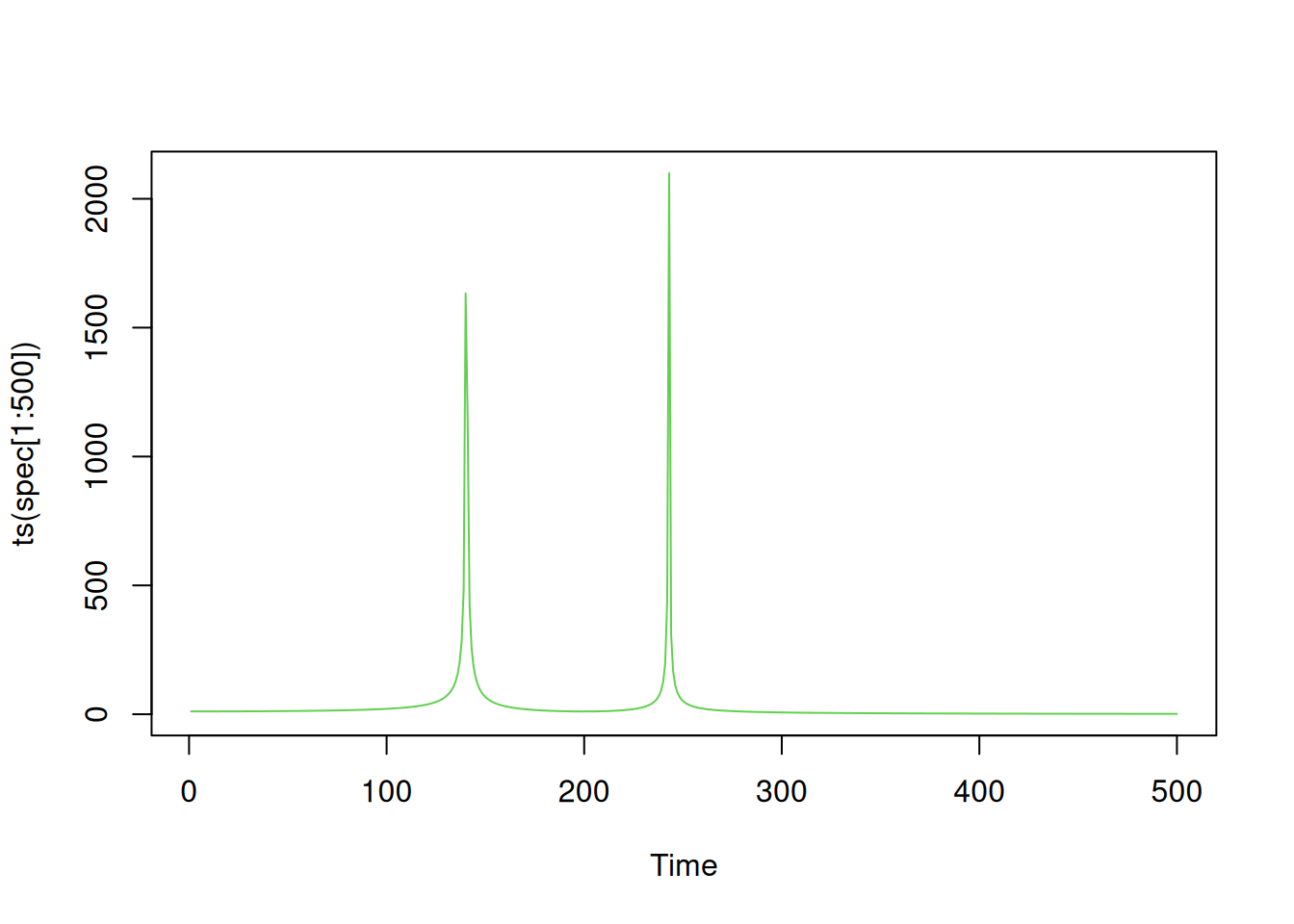

We can clearly see the two peaks in the spectrum corresponding to the row and column frequencies of the dual-tone. The cutoff frequency of 1kHz corresponds to an index of

1000 * length(data) / freq

[1] 200

So we will get the index of the row frequency with

which.max(spec[1:200])

[1] 140

and the index of the column frequency with

200 + which.max(spec[201:500])

[1] 243

These correspond to actual frequencies of

139 * freq / length(data)

[1] 695

242 * freq / length(data)

[1] 1210

So by finding the closest row and column frequencies, we can see that this tone must correspond to the number in the first row and first column. ie. it must be the number “1”.

Task A

Use the sound package to synthesise a sample corresponding to the tones needed to dial your personal mobile phone number. You might want to write a bit of code to semi-automate this. Save the sample as a WAV file, for later use in Task C. Each dual-tone should be exactly 0.2 seconds in duration, and should be followed by a gap of silence of duration 0.1 seconds. If you can, play the sample and check that it “sounds like” a phone number being dialled.

Task B

A mystery phone number can be loaded into R with:

td = tempdir()
fp = file.path(td, "mystery.wav")
if (!file.exists(fp))
  download.file("https://darrenjw.github.io/time-series/extra/mystery.wav", fp)
mysterySamp = loadSample(fp)
mysterySamp

type      : mono
rate      : 44100 samples / second
quality   : 16 bits / sample
length    : 264644 samples
R memory  : 1058576 bytes
HD memory : 529332 bytes
duration  : 6.001 seconds

plot(mysterySamp)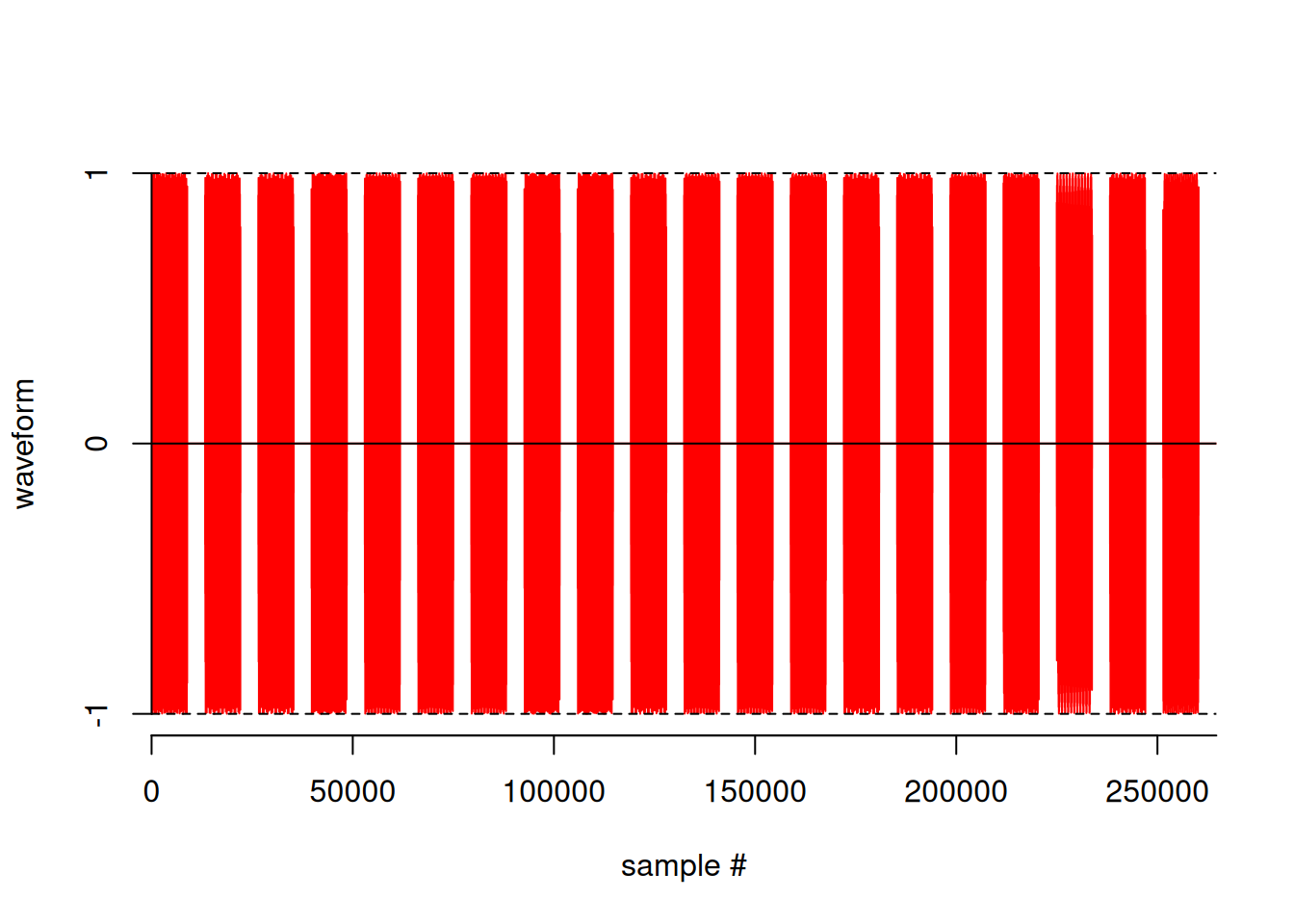

mysteryData = sound(mysterySamp)[1,]
plot(ts(mysteryData, start=0, freq=freq), col=4)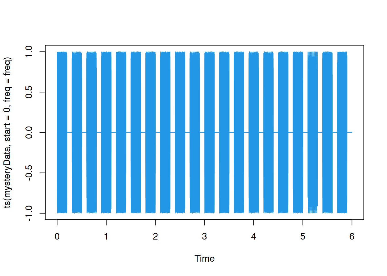

# play(mysterySamp)

The phone number is 20 digits long, and therefore consists of 20 tones. Each tone is exactly 0.2 seconds in duration and followed by a 0.1 second gap of silence.

By extracting each tone in turn and then analysing it with the DFT, figure out the number being dialled. You will almost certainly want to write some code to (semi-)automate this process. Do not dial the number, but if you don’t recognise it, Googling it should reveal if you have figured it out correctly.

Task C (for after the computer practical)

The next time you have access to a regular land-line phone (with a dialling tone), lift the handset (or more likely these days, press the “phone” button) in order to get a dialling tone, then play your WAV file from Task A into the phone’s microphone. If you have completed Task A correctly, your mobile phone should ring.