Many time series exhibit repetitive pseudo-periodic behaviour. It is therefore tempting to try to use (mixtures of) trigonometric functions in order to capture aspects of their behaviour. The weights and frequencies associated with the trig functions will give us insight into the nature of the process. This is the idea behind spectral analysis.
In fact, we know from Fourier analysis that any reasonable function can be described as a mixture of trig functions, so we begin with a very brief recap of Fourier series before thinking about about how to use these ideas in the context of time series models.
5.1.1 Fourier series
Starting from any “reasonable” function, \(f: [-\frac{1}{2},\frac{1}{2}]\rightarrow\mathbb{R}\) (or, equivalently, any periodic function with period 1), we can write \[
f(x) = a_0 + \sum_{k=1}^\infty \left(a_k\cos 2\pi kx + b_k \sin 2\pi kx\right)
\] for coefficients \(a_0, a_1,\ldots,\ b_1, b_2, \ldots\in\mathbb{R}\) to be determined. However, since trig is tricky, it is often more convenient to write this as \[
f(x) = \sum_{k=-\infty}^\infty c_k e^{2\pi\mathrm{i}kx},
\] for \(\ldots,c_{-1},c_0,c_1,\ldots\in\mathbb{C}\). The sum is now doubly-infinite, since we can ensure we get back to a real-valued Fourier series by choosing \(c_{-k} = \bar{c}_k\ \forall\ k\geq 0\) (and hence \(c_0\in\mathbb{R}\)). Now, using the nice orthogonality property \[
\int_{-\frac{1}{2}}^{\frac{1}{2}}e^{2\pi\mathrm{i}(j-k)x}\mathrm{d}x = \delta_{jk} = \begin{cases}1&j=k\\0&\text{otherwise,}\end{cases}
\] we can multiply through our series by \(e^{-2\pi\mathrm{i}jx}\) and integrate to determine the coefficients, \[
c_k = \int_{-\frac{1}{2}}^{\frac{1}{2}} f(x)e^{-2\pi\mathrm{i}kx}\mathrm{d}x.
\] It is a standard (but non-trivial) result of Fourier analysis that this series will converge to \(f(x)\) (in, say, an \(L^2\) sense), for reasonably well-behaved functions, \(f\).
The main point of Fourier series is to represent a periodic (or finite range) function wrt to a countable orthonormal set of (trigonometric) basis functions. But since the mapping is invertible, it just provides us with a mapping back and forth between a function defined on \([-\frac{1}{2},\frac{1}{2}]\) and a countable set of coefficients. So, we could alternatively view this as a way of representing a countable collection of numbers using a function defined on \([-\frac{1}{2},\frac{1}{2}]\). This latter perspective is helpful for the analysis of time series in discrete time, and in this context, the Fourier mapping is known as the discrete time Fourier transform (DTFT).
5.1.2 Discrete time Fourier transform
An infinite time series \(\ldots,x_{-1},x_0,x_1,\ldots\) can be represented by a function \(\hat{x}:[-\frac{1}{2},\frac{1}{2}]\rightarrow\mathbb{C}\) via the relation \[
x_t = \int_{-\frac{1}{2}}^{\frac{1}{2}} \hat{x}(\nu)e^{2\pi\mathrm{i}t\nu}\mathrm{d}\nu,\quad t\in \mathbb{Z},
\] where \[
\hat{x}(\nu) = \sum_{t=-\infty}^\infty x_t e^{-2\pi\mathrm{i}t\nu}.
\]\(\hat{x}(\nu)\) is the weight put on oscillations of frequency \(\nu\). More precisely, \(|\hat{x}(\nu)|\) determines the weight, and \(\operatorname{Arg}[\hat{x}(\nu)]\) determines the phase of the oscillation at that frequency. Note that the sign of the continuous variable (\(\nu\)) has been switched. This doesn’t change anything - it just maintains the usual convention that the forward transform has a minus in the complex exponential and the inverse transform does not. Also note that if the time series is real-valued, then the function \(\hat{x}\) will be Hermitian. That is, it will have the property \(\hat{x}(-\nu) = \overline{\hat{x}(\nu)},\forall \nu\in[0,\frac{1}{2}]\) (and \(\hat{x}(0)\) will be real). Note that no fundamentally new maths is required for this representation - it is just Fourier series turned on its head. That said, there are lots of technical convergence conditions that we are ignoring.
5.2 Spectral representation
Now we have this bijection between discrete-time time series and functions on a unit interval, we can think about what it means for random time series. Clearly a random time series \(X_t\) will induce a random continuous-time process \(\hat{X}(\nu)\), and vice-versa. It will turn out to be very instructive to think about the class of discrete time models induced by a weighted “white noise” process. That is, \(\hat X(\nu) = \sigma(\nu)\eta(\nu)\), where \(\sigma:[-\frac{1}{2},\frac{1}{2}]\rightarrow\mathbb{C}\) is a deterministic function specifying the weight to be placed on the frequency \(\nu\), and \(\eta(\nu)\) is the stationary Gaussian “white noise” process with \(\mathbb{E}[\eta(\nu)]=0\), \(\gamma(\nu) = \delta(\nu)\) (Dirac’s delta). We can therefore represent our random time series as \[
X_t = \int_{-\frac{1}{2}}^{\frac{1}{2}}\sigma(\nu)e^{2\pi\mathrm{i}t\nu}\eta(\nu)\,\mathrm{d}\nu,\quad t\in\mathbb{Z}.
\tag{5.1}\] Now, since \(\eta\) is not a very nice function, it is arguably better to write this as a stochastic integral wrt a Wiener process, \(W\), as \[
X_t = \int_{-\frac{1}{2}}^{\frac{1}{2}}\sigma(\nu)e^{2\pi\mathrm{i}t\nu}\,\mathrm{d}W(\nu),\quad t\in\mathbb{Z},
\] interpreted using Itô calculus. We will largely gloss over this technicality, but writing it this way arguably makes it easier to see that the induced time series will be a Gaussian process. Taking the expectation of Equation 5.1 gives \(\mathbb{E}[X_t]=0\), so then \[\begin{align*}
\mathbb{C}\mathrm{ov}[X_{t+k}, X_{t}]
&= \mathbb{E}[X_{t+k} \bar{X}_{t}] \\
&= \mathbb{E}\left[ \int_{-\frac{1}{2}}^{\frac{1}{2}}\sigma(\nu)e^{2\pi\mathrm{i}(t+k)\nu}\eta(\nu)\,\mathrm{d}\nu \int_{-\frac{1}{2}}^{\frac{1}{2}}\bar{\sigma}(\nu')e^{-2\pi\mathrm{i}t\nu'}\bar{\eta}(\nu')\,\mathrm{d}\nu' \right] \\
&= \mathbb{E}\left[ \int_{-\frac{1}{2}}^{\frac{1}{2}}\mathrm{d}\nu\int_{-\frac{1}{2}}^{\frac{1}{2}}\mathrm{d}\nu'\,\sigma(\nu) \bar{\sigma}(\nu')e^{2\pi\mathrm{i}[(t+k)\nu-t\nu']}\eta(\nu)\bar{\eta}(\nu') \right] \\
&= \int_{-\frac{1}{2}}^{\frac{1}{2}}\mathrm{d}\nu\int_{-\frac{1}{2}}^{\frac{1}{2}}\mathrm{d}\nu\,\sigma(\nu) \bar{\sigma}(\nu)e^{2\pi\mathrm{i}[t(\nu-\nu')+k\nu]}\mathbb{E}[\eta(\nu)\bar{\eta}(\nu')] \\
&= \int_{-\frac{1}{2}}^{\frac{1}{2}}\mathrm{d}\nu\int_{-\frac{1}{2}}^{\frac{1}{2}}\mathrm{d}\nu'\,\sigma(\nu) \bar{\sigma}(\nu')e^{2\pi\mathrm{i}[t(\nu-\nu')+k\nu]}\delta(\nu-\nu') \\
&= \int_{-\frac{1}{2}}^{\frac{1}{2}}\mathrm{d}\nu\,|\sigma(\nu)|^2e^{2\pi\mathrm{i}k\nu} .
\end{align*}\] Since this is independent of \(t\), the induced time series is weakly stationary, with auto-covariance function \[
\gamma_k = \int_{-\frac{1}{2}}^{\frac{1}{2}}|\sigma(\nu)|^2\,e^{2\pi\mathrm{i}k\nu}\,\mathrm{d}\nu.
\] If we define the function \[
S(\nu) \equiv |\sigma(\nu)|^2,
\] then we can re-write this as \[
\gamma_k = \int_{-\frac{1}{2}}^{\frac{1}{2}}S(\nu)\,e^{2\pi\mathrm{i}k\nu}\,\mathrm{d}\nu.
\tag{5.2}\] This is just a discrete time Fourier transform, so we can invert it as \[
S(\nu) = \sum_{k=-\infty}^\infty \gamma_k e^{-2\pi\mathrm{i}k\nu}.
\] The non-negative real-valued function \(S(\nu)\) is known as the spectral density of the discrete time series process. So, glossing over (quite!) a few technical details, essentially any choice of spectral density function leads to a stationary Gaussian discrete time process, and any stationary Gaussian discrete time process has an associated spectral density function. The spectral density function and auto-covariance function are different but equivalent ways of representing the same information. Technical mathematical results relating to this equivalence include the Wiener-Khinchin theorem and Bochner’s theorem. Note that if \(S(\nu)\) is chosen to be an even function, and it typically will, then \[
\gamma_k = 2\int_{0}^{\frac{1}{2}}S(\nu)\,\cos(2\pi k\nu)\,\mathrm{d}\nu,
\] and will be real. Similarly, if \(\gamma_k\) is real (and hence even), as it typically will be, then \[
S(\nu) = \gamma_0 + 2\sum_{k=1}^\infty \gamma_k\cos(2\pi k\nu),
\] and hence is even.
5.2.1 Spectral densities
5.2.1.1 White noise
What discrete time process is represented by a flat spectral density, with \(S(\nu) =\sigma^2,\ \forall \nu\)? Substituting in to Equation 5.2 gives \[
\gamma_k = \begin{cases}\sigma^2&k=0\\0&k>0.\end{cases}
\] In other words, it induces the discrete time white noise process, \(\varepsilon_t\), with noise variance \(\sigma^2\).
5.2.1.2 Some properties of the DTFT
5.2.1.2.1 Linearity
The DTFT is a linear transformation. Suppose that \(z_t = ax_t + by_t\) for some time series \(x_t\) and \(y_t\). Then, \[\begin{align*}
\hat{z}(\nu)
&= \sum_{t=-\infty}^\infty z_t e^{-2\pi\mathrm{i}t\nu} \\
&= \sum_{t=-\infty}^\infty (ax_t + by_t) e^{-2\pi\mathrm{i}t\nu} \\
&= a\sum_{t=-\infty}^\infty x_t e^{-2\pi\mathrm{i}t\nu} + b\sum_{t=-\infty}^\infty y_t e^{-2\pi\mathrm{i}t\nu}\\
&= a\hat{x}(\nu) + b\hat{y}(\nu).
\end{align*}\]
5.2.1.2.2 Time shift
Suppose that \(y_t = Bx_t = x_{t-1}\), for some time series \(x_t\). Then, \[\begin{align*}
\hat{y}(\nu)
&= \sum_{t=-\infty}^\infty y_t e^{-2\pi\mathrm{i}t\nu} \\
&= \sum_{t=-\infty}^\infty x_{t-1} e^{-2\pi\mathrm{i}t\nu} \\
&= e^{-2\pi\mathrm{i}\nu}\sum_{t=-\infty}^\infty x_{t-1} e^{-2\pi\mathrm{i}(t-1)\nu} \\
&= e^{-2\pi\mathrm{i}\nu}\hat{x}(\nu),
\end{align*}\] and more generally, it easily follows that \[
\widehat{B^kx}(\nu) = e^{-2\pi\mathrm{i}k\nu}\hat{x}(\nu).
\]
5.2.1.3 AR(p)
Consider the AR(p) model, \[
X_t - \sum_{k=1}^p \phi_k X_{t-k} = \varepsilon_t,
\] and DTFT both sides. \[\begin{align*}
\hat{X}(\nu) - \sum_{k=1}^p \phi_k e^{-2\pi\mathrm{i}k\nu}\hat{X}(\nu) &= \hat{\varepsilon}(\nu) \\
\Rightarrow \left(1 - \sum_{k=1}^p \phi_k e^{-2\pi\mathrm{i}k\nu}\right)\hat X(\nu) = \hat{\varepsilon}(\nu) \\
\Rightarrow \phi(e^{-2\pi\mathrm{i}\nu})\hat X(\nu) = \hat{\varepsilon}(\nu) \\
\Rightarrow \hat X(\nu) = \frac{\hat{\varepsilon}(\nu)}{\phi(e^{-2\pi\mathrm{i}\nu})}
\end{align*}\] Now, since \(\varepsilon_t\) is a discrete time white noise process, it has a flat spectrum, and we can write \(\hat\varepsilon(\nu) = \sigma\eta(\nu)\), so that \[
\hat X(\nu) = \frac{\sigma}{\phi(e^{-2\pi\mathrm{i}\nu})}\eta(\nu),
\] and from this it is clear that the spectral density of \(X_t\) is given by \[
S(\nu) = \frac{\sigma^2}{|\phi(e^{-2\pi\mathrm{i}\nu})|^2}.
\] Recall that a stationary AR(p) model has roots of \(\phi(z)\) outside of the unit circle. Here, in the denominator, we are traversing around the unit circle, so the spectral density will remain finite for stationary processes.
5.2.1.3.1 Example: AR(2)
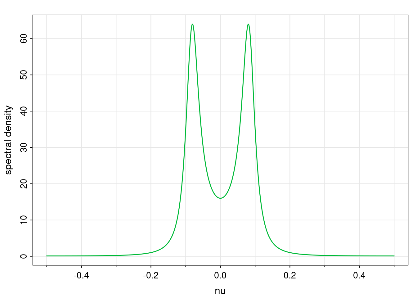
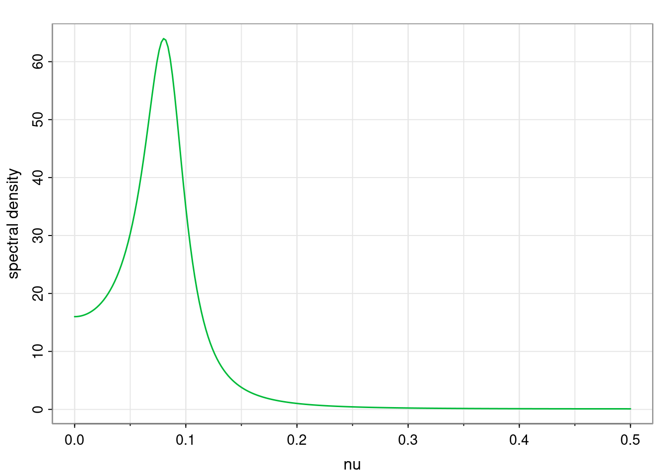
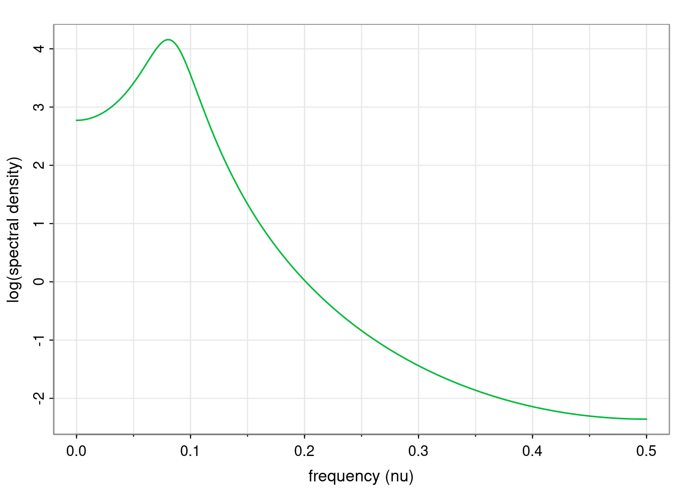
Consider an AR(2) model with \(\phi_1=3/2,\ \phi_2=-3/4,\ \sigma=1\). We can plot the spectral density as follows.
Either way, we see that there is a single strong peak in this spectral density, occurring at around \(\nu=0.08\). In fact, we expect this, since we’ve looked at this AR(2) model previously.
So this model has oscillations with period around 12. This all makes sense, since the spectral density will be largest at points on the unit circle that are closest to the roots of the characteristic polynomial. But this will happen when the argument of the point of the unit circle matches that of a root.
5.2.1.4 ARMA(p,q)
A very similar argument to that used for AR(p) models confirms that the spectral density of an ARMA(p,q) process is given by \[
S(\nu) = \sigma^2\frac{|\theta(e^{-2\pi\mathrm{i}\nu})|^2}{|\phi(e^{-2\pi\mathrm{i}\nu})|^2}.
\] Note that when calculating spectral densities by hand it can be useful to write this in the form \[
S(\nu) = \sigma^2\frac{\theta(e^{2\pi\mathrm{i}\nu})\theta(e^{-2\pi\mathrm{i}\nu})}{\phi(e^{2\pi\mathrm{i}\nu})\phi(e^{-2\pi\mathrm{i}\nu})},
\] and to simplify the numerator and denominator separately, recognising the resulting real-valued trig functions that must arise, since both the numerator and denominator are real.
5.3 Finite time series
Of course, in practice we do not work with time series of infinite length. We instead work with time series of finite length, \(n\). In the context of spectral analysis, it is more convenient to work with zero-based indexing, so we write our time series as \[
x_0,x_1,\ldots,x_{n-1}.
\] Since we only have \(n\) degrees of freedom, we do not need a continuous function \(\hat x(\nu)\) in order to fix them. Since everything is linear, knowing \(\hat x(\nu)\) at just \(n\) points would be sufficient, since that would give us \(n\) linear equations in \(n\) unknowns. Knowing it at \(n\) equally spaced points around the unit circle is natural, and turns out to give nice orthogonality properties that make everything very neat. This is the idea behind the discrete Fourier transform (DFT).
5.3.1 The discrete Fourier transform
The (forward) DFT takes the form \[
\hat{x}_k = \sum_{t=0}^{n-1} x_t e^{-2\pi\mathrm{i}kt/n},\quad k=0,1,\ldots,n-1.
\] It can be inverted with \[
x_t = \frac{1}{n} \sum_{k=0}^{n-1} \hat{x}_k e^{2\pi\mathrm{i}kt/n},\quad t=0,1,\ldots,n-1.
\] For the DTFT, the integral traversed the unit circle clockwise starting from minus one. The DFT moves around the unit circle clockwise starting from one, but this is just a commonly used convention, and doesn’t change anything fundamental about the transform. These transforms are simple finite linear sums mapping back and forth between \(n\) values in the time and frequency domains, and hence are very amenable to computer implementation.
To understand how it works, it is helpful to define \(\omega=e^{2\pi\mathrm{i}/n}\), the \(n\)th root of unity, with \(w^n=1\) and \(\overline{\omega^k} = \omega^{-k} = \omega^{n-k}\). We can then write the transforms slightly more neatly as \[
x_t = \frac{1}{n}\sum_{k=0}^{n-1}\hat{x}_k \omega^{kt} \quad \text{and} \quad
\hat{x}_k = \sum_{t=0}^{n-1} x_t \omega^{-kt}.
\] That the inversion works follows from the nice orthogonality property, \[
\sum_{t=0}^{n-1} \omega^{jt}\omega^{-kt} = \sum_{t=0}^{n-1} \omega^{(j-k)t} = n\,\delta_{jk},
\] which follows from the fact that the roots of unity sum to zero. If we start from the definition of \(x_t\) and sub in for the definition of \(\hat{x}_k\) we find \[\begin{align*}
\frac{1}{n}\sum_{k=0}^{n-1}\hat{x}_k\omega^{kt}
&= \frac{1}{n}\sum_{k=0}^{n-1} \sum_{s=0}^{n-1}x_s\omega^{-ks} \omega^{kt} \\
&= \frac{1}{n}\sum_{s=0}^{n-1} x_s \sum_{k=0}^{n-1}\omega^{-ks} \omega^{kt} \\
&= \frac{1}{n}\sum_{s=0}^{n-1} x_s n \delta_{st} \\
&= x_t,
\end{align*}\] as required. The factor of \(n\) in the inverse is a bit annoying, but has to go somewhere. The convention that we have adopted is the most common, but there are others.
The finite, discrete and linear nature of the DFT (and its inverse) make it extremely suitable for computer implementation. Naive implementation would involve \(\mathcal{O}(n)\) operations to compute each coefficient, and hence a full transform would involve \(\mathcal{O}(n^2)\) operations. However, it turns out that a divide-and-conquer approach can be used to reduce this to \(\mathcal{O}(n\log n)\) operations. The algorithm that implements the DFT with reduced computational complexity is known as the fast Fourier transform (FFT). For large time series, this difference in complexity is transformational, and is one of the reasons that the FFT (and the very closely related discrete cosine transform, DCT) now underpin much of modern life.
5.3.1.1 The FFT in R
R has a built-in fft function that can efficiently compute a DFT. It can also invert the DFT, but it returns an unnormalised inverse (without the factor of \(n\)), so it is convenient to define our own function to invert the DFT.
It can also be instructive to consider the DFT in matrix-vector form. Starting with the inverse DFT, we can write this as \[
\mathbf{x} = \frac{1}{n} \mathsf{F}_n \hat{\mathbf x},
\] where \(\mathsf{F}_n\) is the \(n\times n\) Fourier matrix with \((i,j)\)th element \(w^{ij}\). Clearly \(\mathsf{F}_n\) is symmetric (\(\mathsf{F}_n^\top= \mathsf{F}_n\)). Now notice that the forward DFT is just \[
\hat{\mathbf x} = \bar{\mathsf{F}}_n \mathbf{x}
\] Further, our orthogonality property implies that \(\mathsf{F}_n \bar{\mathsf{F}}_n = n\mathbb{I}\) (so \(\mathsf{F}_n\) is unitary, modulo a factor of \(n\)), and \(\mathsf{F}_n^{-1} = \bar{\mathsf{F}}_n/n\). So inversion is now clear, since if we start with the definition of \(\mathbf{x}\) and substitute in for \(\hat{\mathbf x}\), we get \[
\frac{1}{n}\mathsf{F}_n\hat{\mathbf x} = \frac{1}{n}\mathsf{F}_n \bar{\mathsf{F}}_n \mathbf{x} = \frac{1}{n}n\mathbb{I}\mathbf{x} = \mathbf{x},
\] as required.
5.3.2 The periodogram
For a time series \(x_0,x_1,\ldots,x_{n-1}\) with DFT \(\hat{x}_0,\hat{x}_1,\ldots,\hat{x}_{n-1}\), the periodogram is just the sequence of non-negative real numbers \[
I_k = |\hat{x}_k|^2, \quad k=0,1,\ldots,n-1.
\] They represent a (very bad) estimate of the spectral density function.
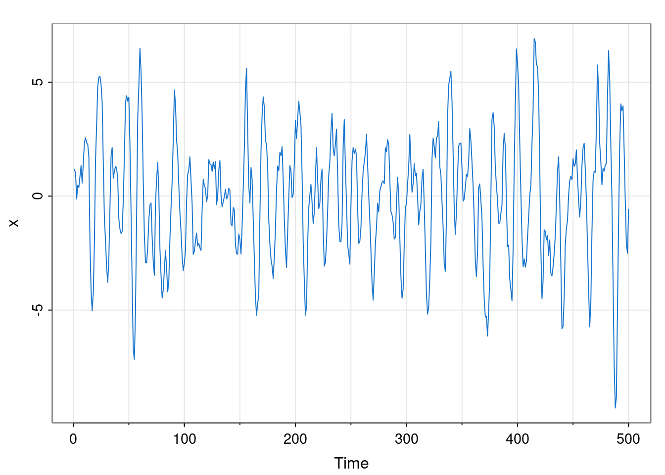
5.3.2.1 Example: AR(2)
Let’s see how this works in the context of our favourite AR(2) model. First, simulate some data from the model.
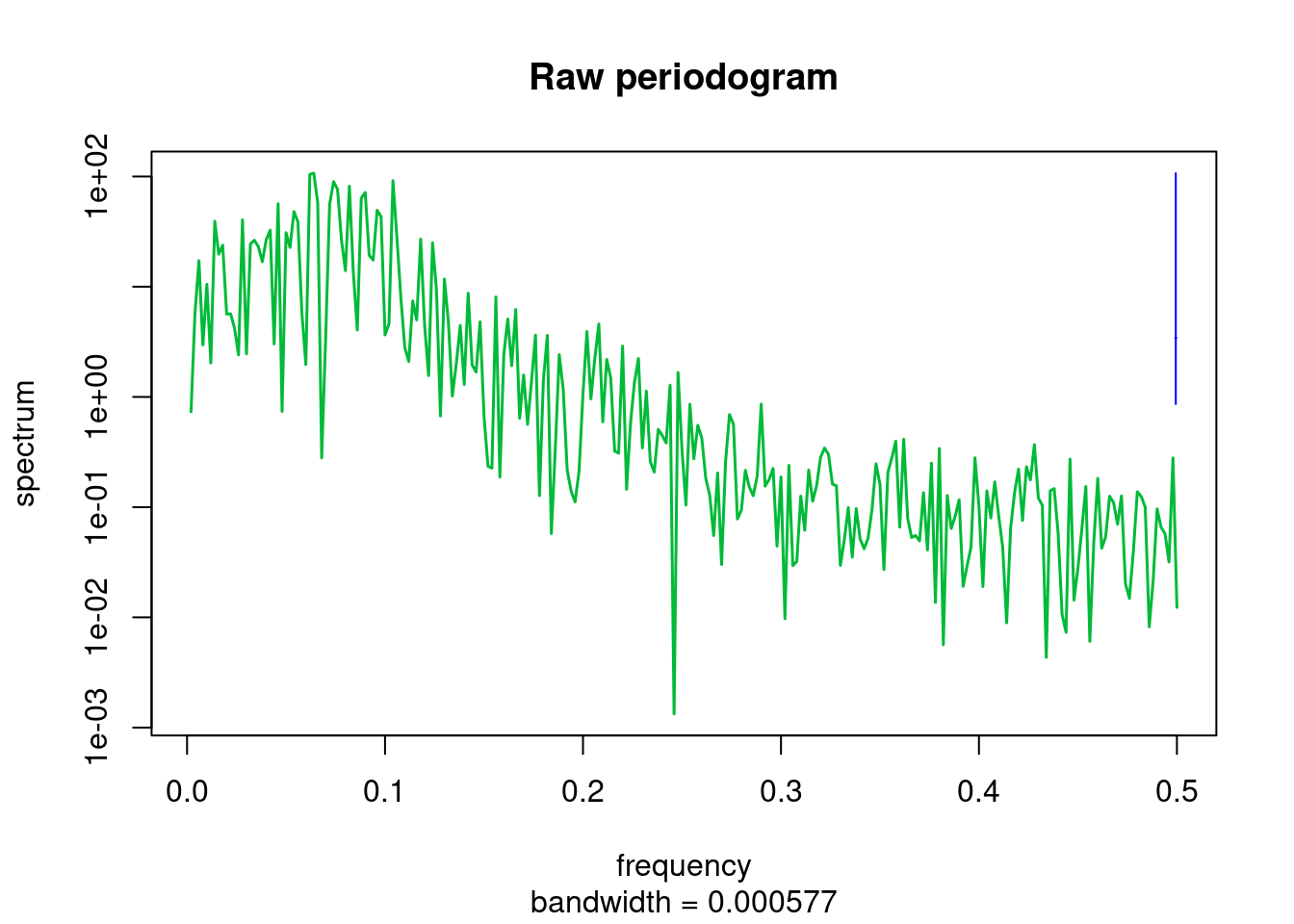
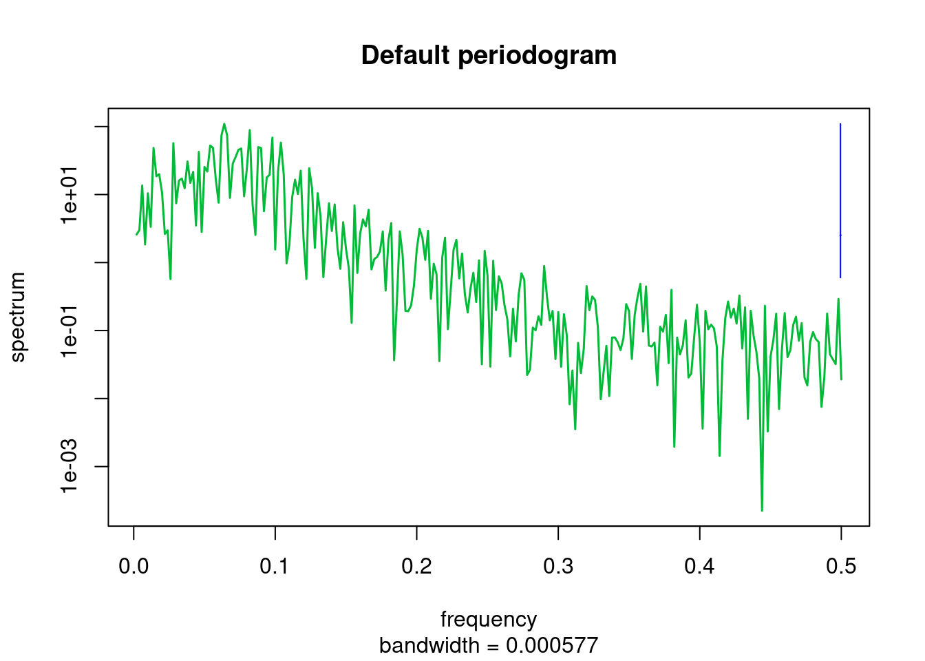
This is now exactly like R’s built-in periodogram function, spec.pgram, with all “tweaks” disabled. But the default periodogram does a little bit of pre-processing.
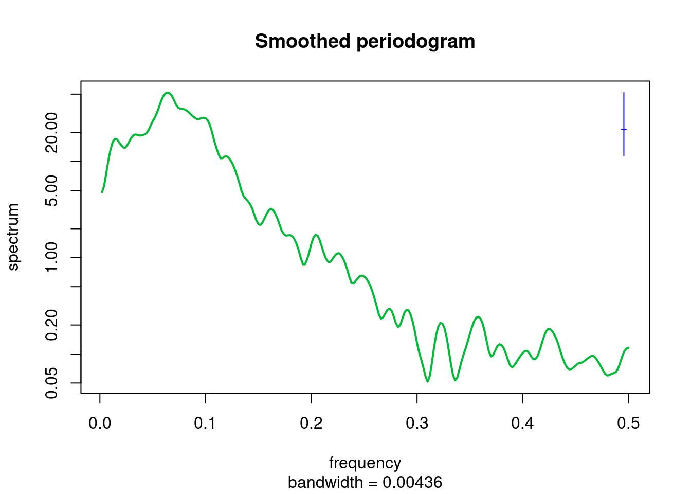
In practice, various smoothing methods are used to get better a better estimate of the spectral density. This is the subject of spectral density estimation, but the details of this do not concern us. In the final plot, a peak at a frequency of around 0.08 can be seen, as we would hope.
5.3.3 Smoothing with the DFT
The potential applications of the DFT (and of spectral analysis, more generally) are many and varied, but we don’t have time to explore them in detail here. But essentially, the DFT decomposes your original signal into different frequency components. These different frequency components can be separated, manipulated and combined in various ways. One obvious application is smoothing, where high frequency components are simply wiped out. This is best illustrated by example.
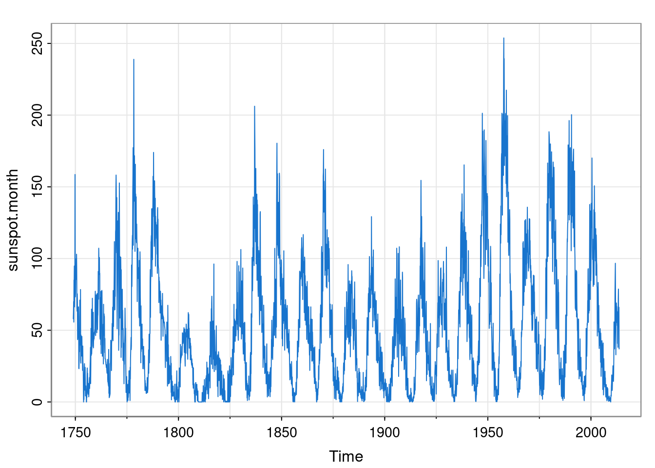
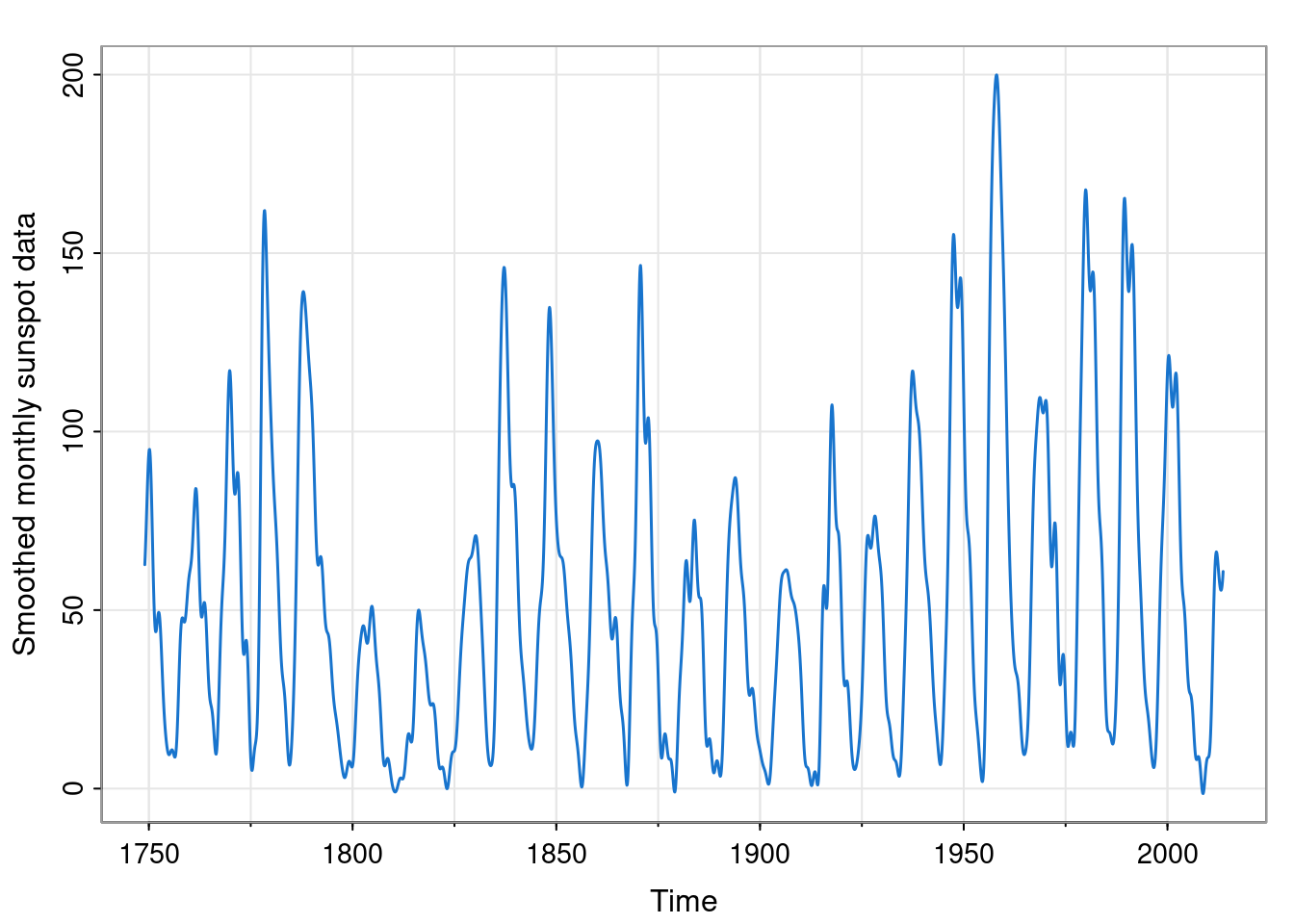
5.3.3.1 Example: monthly sunspot data
We previously looked at yearly sunspot data, and fitted an AR(2) model to it. There is also a monthly sunspot dataset that is in many ways more interesting.
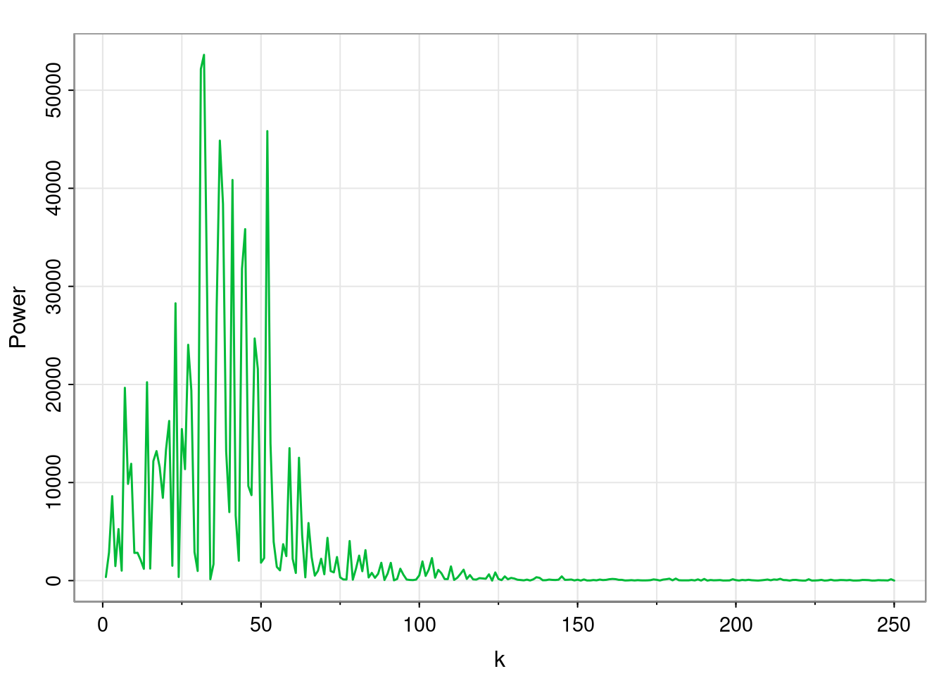
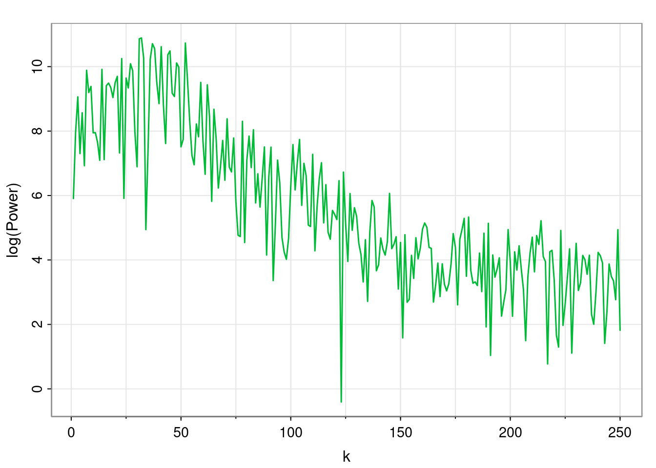
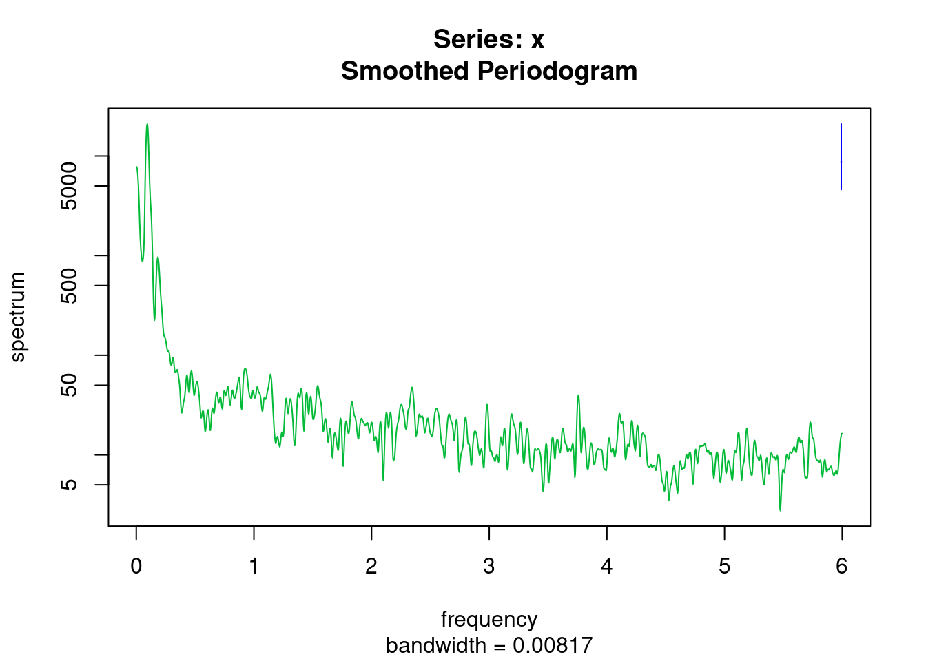
We can see strong oscillations with period just over a decade. However, fitting an AR(2) to this data fails miserably due to the presence of strong high frequency oscillations. A quick look at the periodogram
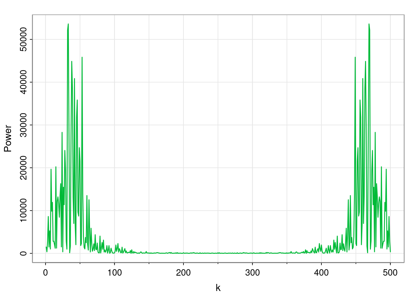
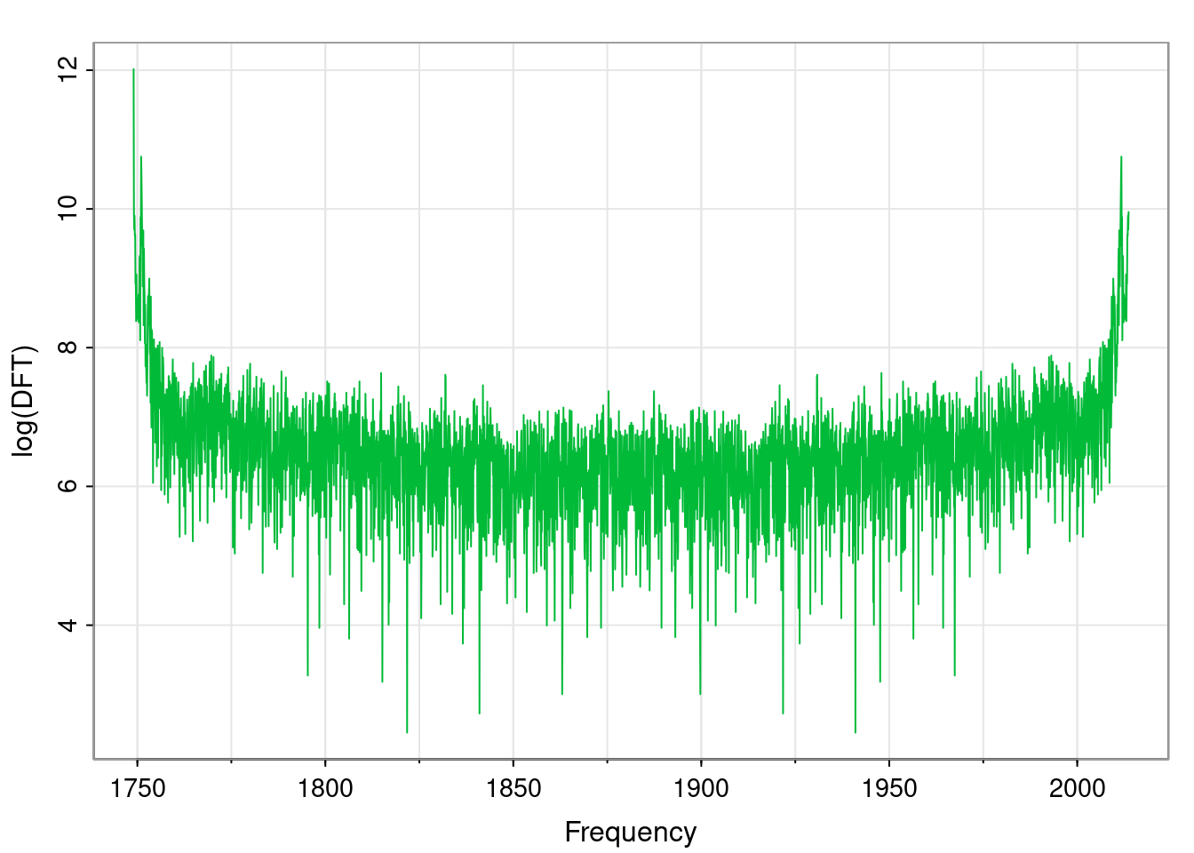
reveals that although there is a strong peak at low frequency oscillation, there is also a lot of higher frequency stuff going on. So, let’s look more carefully at the DFT of the data.
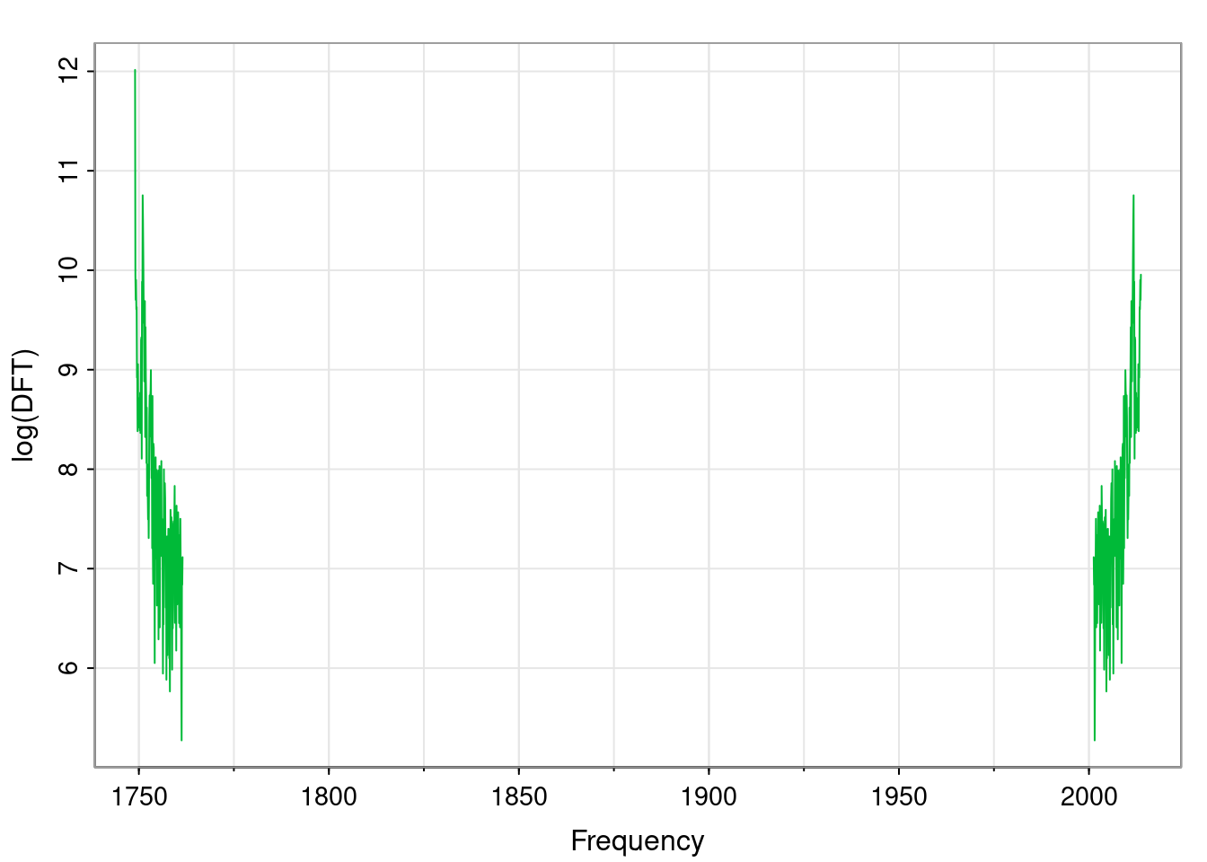
The peaks close to the two ends correspond to the low frequency oscillations that we are interested in. Everything in the middle is high frequency noise that we are not interested in, so let’s just get rid of it. Suppose that we want to keep the first (and last) 150 frequency components. We can zero out the rest as follows.