Random number generation

5.1 Simple generators and what can go wrong

Since the 1950s there has been much work on linear congruential generators. The intuitive motivation is something like this. Suppose I take an integer, multiply it by some enormous factor, re-write it in base - ‘something huge’, and then throw away everything except for the digits after the decimal point. Pretty hard to predict the result, no? So, if I repeat the operation, feeding each step’s output into the input for the next step, a more or less random sequence might result. Formally the pseudorandom sequence is defined by

where $b$ is 0 or 1, in practice. This is started with a seed $X_0$. The $X_ i$ are integers ($<M$, of course), but we can define $U_ i = X_ i/M$. Now the intuitive hope that this recipe might lead to $U_ i$ that are reasonably well modelled by i.i.d. $U(0,1)$ r.v.s is only realised for some quite special choices of $a$ and $M$, and it takes some number theory to give the generator any sort of theoretical foundation (see Ripley, 1987, Chapter 2).

An obvious property to try to achieve is full period. We would like the generator to visit all possible integers between $1-b$ and $M-1$ once before it starts to repeat itself (clearly the first time it revisits a value, it starts to repeat itself). We would also like successive $U_ i$s to appear uncorrelated. A notorious and widely used generator called RANDU, supplied at one time with IBM machines, met these basic considerations with

This appears to do very well in 1 dimension.

n <- 100000 ## code NOT for serious use
x <- rep(1,n)
a <- 65539;M <- 2^31;b <- 0 ## Randu
for (i in 2:n) x[i] <- (a*x[i-1]+b)%%M
u <- x/(M-1)

qqplot((1:n-.5)/n,sort(u))

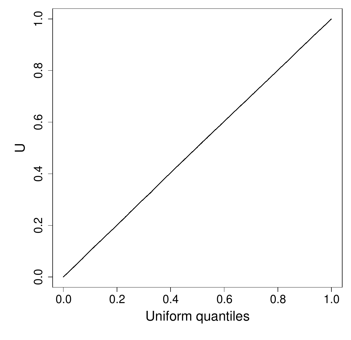
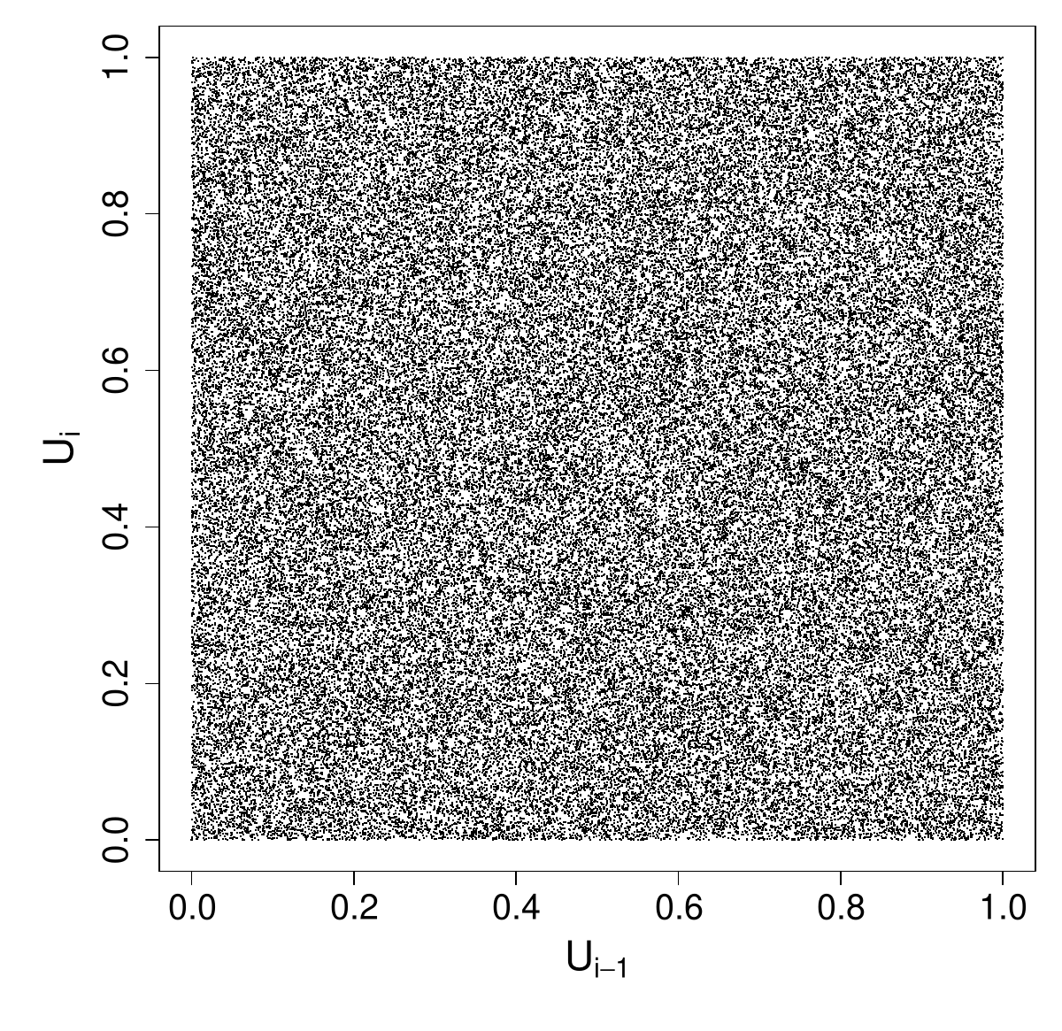
Similarly a 2D plot of $U_ i$ vs $U_{i-1}$ indicates no worries with serial correlation

## Create data frame with U at 3 lags...
U <- data.frame(u1=u[1:(n-2)],u2=u[2:(n-1)],u3=u[3:n])

plot(U$u1,U$u2,pch=".")

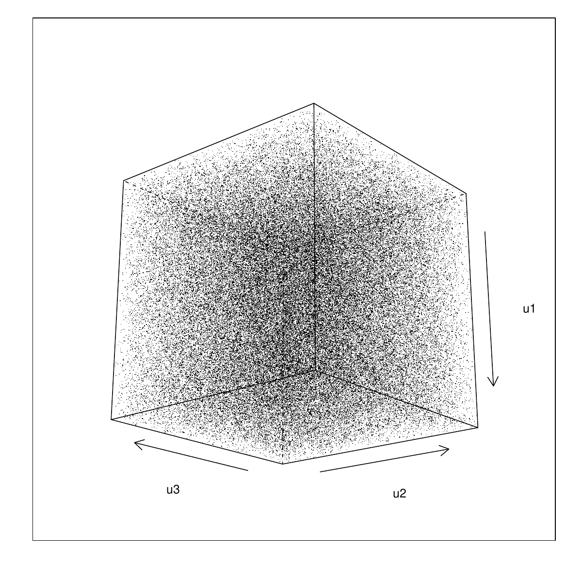
We can also check visually what the distribution of the triples $(U_ i, U_{i-1},U_{i-2})$ looks like.

library(lattice)
cloud(u1~u2*u3,U,pch=".",col=1,screen=list(z=40,x=-70,y=0))

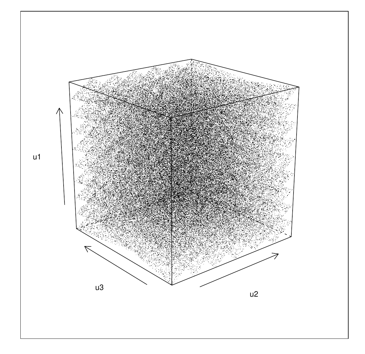
…not quite so random looking. Experimenting a little with rotations gives

cloud(u1~u2*u3,U,pch=".",col=1,screen=list(z=40,x=70,y=0))

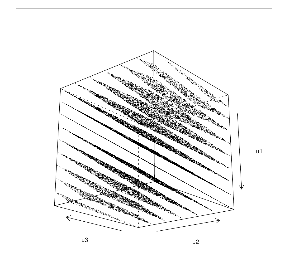
i.e. the triples lie on one of 15 planes. Actually you can show that this must happen (see Ripley, 1987, section 2.2).

Does this deficiency matter in practice? When we looked at numerical integration we saw that quadrature rules based on evaluating integrands on fixed lattices become increasingly problematic as the dimension of the integral increases. Stochastic integration overcomes the problems by avoiding the biases associated with fixed lattices. We should expect problems if we are performing stochastic integration on the basis of random numbers that are in fact sampled from some coarse lattice.

So the first lesson is to use generators that have been carefully engineered by people with a good understanding of number theory, and have then been empirically tested (Marsaglia’s Diehard battery of tests provides one standard test set). For example, if we stick with simple congruential generators, then

is a much better bet. Here is its triples plot. No amount of rotating provides any evidence of structure.

Although this generator is much better than RANDU, it is still problematic. An obvious infelicity is the fact that a very small $X_ i$ will always be followed by an unusually small $X_{i+1}$ (consider $X_ i = 1$, for example). This is not a property that would be desirable in a time series simulation, for example. Not quite so obvious is the fact that for any congruential generator of period $M$, then $k-$tuples, $U_ i, U_{i-1}, \ldots , U_{i-k+1}$ will tend to lie on a finite number of $k-1$ dimensional planes (e.g. for RANDU we saw 3-tuples lying on 2 dimensional planes.) There will be at most $M^{1/k}$ such planes, and as RANDU shows, there can be far fewer. The upshot of this is that if we could visualise 8 dimensions, then the 8-tuple plot for (5.1) would be just as alarming as the 3D plot was for RANDU. 8 is not an unreasonably large dimension for an integral.

Generally then, it might be nice to have generators with better behaviour than simple congruential generators, and in particular we would like generators where $k-$tuples appear uniformly distributed on $[0,1]^ k$ for as high a $k$ as possible (referred to as having a high k-distribution).

5.2 Building better generators

An alternative to the congruential generators are generators which focus on generating random sequences of 0s and 1s. In some ways this seems to be the natural fundamental random number generation problem when using modern digital computers, and at time of writing it also seems to be the approach that yields the most satisfactory results. Such generators are often termed shift-register generators. The basic approach is to use bitwise binary operations to make a binary sequence ‘scramble itself’. An example is Marsaglia’s (2003) Xorshift generator as recommended in Press et al. (2007).

Let $x$ be a 64-bit variable (i.e. an array of 64 0s or 1s). The generator is initialised by setting to any value (other than 64 0s). The following steps then constitute one iteration (update of $x$)

each iteration generates a new random sequence of 0s and 1s. $\wedge$ denotes ‘exclusive or’ (XOR) and $>>$ and $<<$ are right-shift and left shift respectively, with the integers $a, b$ and $c$ giving the distance to shift. $a=21$, $b=35$ and $c=4$ appear to be good constants (but see Press et al., 2007, for some others).

If you are a bit rusty on these binary operators then consider an 8-bit example where x=10011011 and z=01011100.

• x<<1 is 00110110, i.e. the bit pattern is shifted leftwards, with the leftmost bit discarded, and the rightmost set to zero.

• x<<2 is 01101100, i.e. the pattern is shifted 2 bits leftwards, which also entails discarding the 2 leftmost bits and zeroing the two rightmost.

• x>>1 is 01001101, same idea, but rightwards shift.

• x^z is 11000111, i.e. a 1 where the bits in x and z disagree, and a 0 where they agree.

The Xorshift generator is very fast, has a period of $2^{64}-1$, and passes the Diehard battery of tests (perhaps unsurprising as Marsaglia is responsible for that too). These shift register generators suffer similar granularity problems to congruential generators (there is always some $k$ for which $[0,1]^ k$ can not be very well covered by even $2^{64}-1$ points), but tend to have all bit positions ‘equally random’, whereas lower order bits from congruential generator sequences often have a good deal of structure.

Now we reach a fork in the road. To achieve better performance in terms of longer period, larger k-distribution, and fewer low order correlation problems, there seem to be two main approaches, the first pragmatic, and the second more theoretical.

1. 1.

   Combine the output from several ‘good’, well understood, simple generators using operations that maintain randomness (e.g. XOR and addition, but not multiplication). When doing this, the output from the combined generators is never fed back into the driving generators. Preferably combine rather different types of generator. Press et al. (2007) make a convincing case for this approach. Wichmann-Hill, available in R is an example of such a combined generator, albeit based on 3 very closely related generators.

2. 2.

   Use more complicated generators — non-linear or with a higher dimensional state that just a single $X_ i$ (see Gentle, 2003). For example, use a shift register type generator based on maintaining the history of the last $n$ bit-patterns, and using these in the bit scrambling operation. Matsumoto and Nishimura’s (1998) Mersenne Twister is of this type. It achieves a period of $2^{19937}-1$ (that’s not a misprint: $2^{19937}-1$ is a ‘Mersenne prime’ ¹ ), and is 623-distributed at 32 bit accuracy. i.e. its 623-tuples appear uniformly distributed (each appearing the same number of times in a full period) and spaced $2^{-32}$ apart (without the ludicrous period this would not be possible). It passes Diehard, is the default generator in R, and C source code is freely available.

5.3 Uniform generation conclusions

I hope that the above has convinced you that random number generation, and use of pseudo-random numbers are non-trivial topics that require some care. That said, most of the time, provided you pick a good modern generator, you will probably have no problems. As general guidelines…

1. 1.

   Avoid using black-box routines supplied with low level languages such as C, you don’t know what you are getting, and there is a long history of these being botched.

2. 2.

   Do make sure you know what method is being used to generate any uniform random deviates that you use, and that you are satisfied that it is good enough for purpose.

3. 3.

   For any random number generation task that relies on $k-$tuples having uniform distribution for high $k$ then you should be particularly careful about what generator you use. This includes any statistical task that is somehow equivalent to high dimensional integration.

4. 4.

   The Mersenne Twister is probably the sensible default choice in most cases, at present. For high dimensional problems it remains a good idea to check answers with a different high-quality generator. If results differ significantly, then you will need to find out why (probably starting with the ‘other’ generator).

Note that I haven’t discussed methods used by cryptographers. Cryptographers want to use (pseudo)random sequences of bits (0s and 1s) to scramble messages. Their main concern is that if someone were to intercept the random sequence, and guess the generator being used, they should not be able to infer the state of the generator. Achieving this goal is quite computer intensive, which is why generators used for cryptography are usually over engineered for simulation purposes.

5.4 Other deviates

Once you have a satisfactory stream of i.i.d. $U(0,1)$ deviates then generating deviates from other standard distributions is much more straightforward. Conceptually, the simplest approach is inversion. We know that if $X$ is from a distribution with continuous c.d.f. $F$ then $F(X)\sim U(0,1)$. Similarly, if we define the inverse of $F$ by $F^-(u) = {\rm min}(x|F(x)\ge u)$, and if $U\sim U(0,1)$, then $F^-(U)$ has a distribution with c.d.f. $F$ (this time with not even a continuity restriction on $F$ itself).

As an example here is inversion used to generate 1 million i.i.d. $N(0,1)$ deviates in R.

  system.time(X <- qnorm(runif(1e6)))

##    user  system elapsed 
##   0.051   0.000   0.051

For most standard distributions (except the exponential) there are better methods than inversion, and the happy situation exists where textbooks tend to agree what these are. Ripley’s (1987) Chapter 3 is a good place to start, while the lighter version is provided by Press et al. (2007) Chapter 7. R has many of these methods built in. For example an alternative generation of 1 million i.i.d. $N(0,1)$ deviates would use.

  system.time(Z <- rnorm(1e6))

##    user  system elapsed 
##    0.06    0.00    0.06

5.5 Further reading on pseudorandom numbers

• Gentle, J.E. (2003) Random Number Generation and Monte Carlo Methods (2nd ed), Springer, Chapters 1 and 2 provides up to date summaries both of uniform generators, and of generator testing. Chapter 3 covers Quasi Monte Carlo, and the remaining chapters cover simulation from other distributions + software.

• Matsumoto, M. and Nishimura, T. (1998) Mersenne Twister: A 623-dimensionally equidistributed uniform pseudo-random number generator, ACM Transactions on Modeling and Computer Simulation, 8, 3-30. This gives details and code for the Mersenne Twister.

• http://www.math.sci.hiroshima-u.ac.jp/~m-mat/MT/emt.html gives the Mersenne Twister source code.

• Marsaglia, G. (2003) Xorshift RNGs, Journal of Statistical Software, 8(14):1-6.

• DIEHARD is George Marsaglia’s Diehard battery of tests for random number generators: https://en.wikipedia.org/wiki/Diehard_tests

• Press, W.H., S.A. Teukolsky, W.T. Vetterling and B.P Flannery (2007) Numerical Recipes (3rd ed.) Cambridge. Chapter 7, on random numbers is good and reasonably up to date, but in this case you do need the third edition, rather than the second (and certainly not the first).

• Ripley (1987, re-issued 2006) Stochastic Simulation, Wiley. Chapter’s 2 and 3 are where to go to really get to grips with the issues surrounding random number generation. The illustrations alone are an eye opener. You probably would not want to use any of the actual generators discussed and the remarks about mixed generators now look dated, but the given principles for choosing generators remain sound (albeit with some updating of what counts as simple, and the integers involved). See chapter 3 and 4 for simulating from other distributions, given uniform deviates.

• Gamerman, D. and H.F. Lopes (2006) Markov Chain Monte Carlo: Stochastic simulation for Bayesian inference, CRC. Chapter 1 has a nice compact introduction to simulation, given i.i.d. $U(0,1)$ deviates.

• Devroye, L., (2003) Non-Uniform Random Variate Generation, Springer. This is a classic reference. Now out of print, it is available on-line. http://www.nrbook.com/devroye/

• Steele Jr, Guy L., Doug Lea, and Christine H. Flood. "Fast splittable pseudorandom number generators." ACM SIGPLAN Notices 49.10 (2014): 453-472. In the context of parallel computing, sequential random number generators are very problematic. Splittable generators turn out to be very useful in this context.