Pre-course material, 2022/23
Originally by Simon Wood (2013), updated by Finn Lindgren (2014, 2016, 2017), and
Darren Wilkinson (2018, 2019, 2020, 2022)
1 Introduction
The APTS Statistical Computing course aims to introduce some rudiments of numerical analysis, which it is helpful to know in order to do good statistics research. To get the most out of the course you need to arrive with a reasonable knowledge of undergraduate statistics/mathematics (see next section), and you need to be able to do some basic R programming.
If you do not have good prior knowledge of R then you should work through Ruth Ripley’s R programming for APTS students notes at:
http://portal.stats.ox.ac.uk/userdata/ruth/APTS2013/APTS.html
before these notes. If you are fluent in R it is still a good idea to look through the notes, even if only briefly (Q8 in Section 4 is easier if you do). Once you are sufficiently well prepared in R programming, Section 4, below, provides some orientation exercises using R, designed to help you get the most out of the Statistical Computing module. If you can complete the exercises reasonably well, then you are likely to be well prepared for the course. Some pointers to other material on R are also given, along with a list of mathematical and statistical things that the course assumes you already know.
A reasonable attempt at at least exercises 1 through 4 in Section 4 is essential in order to get the most out of the lab sessions during the APTS week. Just being comfortable that in principle you could do them is not enough in this case. Your solutions to the exercises may help with the labs.
For the lab sessions it will be assumed that you have access to an internet-connected computer running R, and that you can install R packages on it.
R is available from http://cran.r-project.org. It’s also highly recommended to have RStudio installed (http://posit.co/).
2 Mathematical and statistical preliminaries
Here is a check-list of basic mathematical/statistical concepts that it might help to brush up on if you are a little rusty on any of them.
-
1.
The multivariate version of Taylor’s theorem.
-
2.
The chain rule for differentiation.
-
3.
The multivariate normal distribution and its p.d.f.
-
4.
Linear models and the notion of a random effect.
-
5.
How to multiply matrices (by each other and with vectors). Matrix addition.
-
6.
The meaning of: square matrix, matrix transposition; upper/lower triangular matrix; symmetric matrix; diagonal matrix; trace of a matrix; identity matrix; positive (semi-) definite matrix.
-
7.
The notion of a matrix inverse and its relationship to solving the matrix equation for , where is a square matrix and and are vectors.
-
8.
The definition of eigenvectors and eigenvalues.
-
9.
The determinant of a matrix.
-
10.
Orthogonal matrices. The fact that if is an orthogonal matrix then is a rotation/reflection of vector .
-
11.
The rank of a matrix and the problems associated with not being full rank.
Most textbooks with titles like ‘Mathematics for Engineers/Scientists/Science students’ will provide all that is necessary: pick the one you like best, or is nearest to hand. At time of writing, the Wikipedia entries on the above material looked fairly reasonable (http://en.wikipedia.org/wiki/).
The course will assume that you know the following basic matrix terminology:
3 Getting help with R
If you are not already familiar with R then work through the R programming for APTS students notes at
http://portal.stats.ox.ac.uk/userdata/ruth/APTS2013/APTS.html before doing anything else. In fact, even if you are an expert in R, the notes are worth reviewing.
Here are some pointers to further information…
-
There is a large amount of free documentation available. An introduction to R at is a good place to start. See http://cran.r-project.org/manuals.html.
-
http://cran.r-project.org/other-docs.html is also worth a look.
-
For books on R see http://www.r-project.org/doc/bib/R-books.html.
-
From the R command line typing
help.start()will launch an html version of the R help system: this is probably the best way to access the online help when starting out.
4 Some exercises
The solutions to these exercises will appear on the APTS web site one week before the start of the course. You will get most out of the exercises by attempting them before looking at the solutions.
-
1.
Computers do not represent most real numbers exactly. Rather, a real number is approximated by the nearest real number that can be represented exactly (floating point number), given some scheme for representing real numbers as fixed length binary sequences. Often the approximation is not noticeable, but it can make a big difference relative to exact arithmetic (imagine that you want to know the difference between 2 distinct real numbers that are approximated by the same binary sequence, for example).
One consequence of working in finite precision arithmetic is that for any number , there is a small number for which is indistinguishable from (with any number smaller than this having the same property).
-
(a)
Try out the following code to find the size of this number, when .
eps <- 1
x <- 1
while (x+eps != x) eps <- eps/2
eps/x
-
(b)
Confirm that the final eps here is close to the largest for which and give rise to the same floating point number.
-
(c)
2*epsis stored in R as.Machine$double.eps. Confirm this. -
(d)
Confirm that you get the same eps/x value for x = 1/8,1/4,1/2,1,2, 4 or 8.
-
(e)
Now try some numbers which are not exactly representable as modest powers of 2, and note the difference.
-
(f)
In terms of decimal digits, roughly how accurately are real numbers numbers being represented here?
-
(a)
-
2.
R is an interpreted language. Instructions are interpreted ‘on the fly’. This tends to mean that it is efficient to code in such a way that many calculations are performed per interpreted instruction. Often this implies that loops should be avoided, otherwise R can spend much more time interpreting the instructions to carry out a calculation than on performing the calculation itself.
-
(a)
Re-write the following to eliminate the loops, first using apply and then using rowSums
Confirm that all three versions give the same answers, but that your re-writes are much faster than the original. (system.time is a useful function.)X <- matrix(runif(100000),1000,100) z <- rep(0,1000) for (i in 1:1000) { for (j in 1:100) z[i] <- z[i] + X[i,j] }
-
(b)
Re-write the following, replacing the loop with efficient code.
Confirm that your re-write is faster but gives the same result.n <- 100000 z <- rnorm(n) zneg <- 0;j <- 1 for (i in 1:n) { if (z[i]<0) { zneg[j] <- z[i] j <- j + 1 } }
Note that while it is important to avoid loops which perform a few computationally cheap operations at each step, little will be gained by removing loops where each pass of the loop is itself irreducibly expensive.
-
(a)
-
3.
Run the following code
Evaluate , and where is the diagonal matrix such that .set.seed(1) n <- 1000 A <- matrix(runif(n*n),n,n) x <- runif(n)
-
4.
Consider solving the matrix equation for , where is a known vector and a known matrix. The formal solution to the problem is , but it is possible to solve the equation directly, without actually forming . This question will explore this a little. Read the help file for solve before trying it.
-
(a)
First create an , and satisfying .
The idea is to experiment with solving the for , but with a known truth to compare the answer to.set.seed(0) n <- 5000 A <- matrix(runif(n*n),n,n) x.true <- runif(n) y <- A%*%x.true
-
(b)
Using solve form the matrix explicitly, and then form . Note how long this takes. Also assess the mean absolute difference between x1 and x.true (the approximate mean absolute ‘error’ in the solution).
-
(c)
Now use solve to directly solve for without forming . Note how long this takes and assess the mean absolute error of the result.
-
(d)
What do you conclude?
-
(a)
-
5.
The empirical cumulative distribution function for a set of measurements is
where denotes ‘number of values less than ’.
When answering the following, try to ensure that your code is commented, clearly structured, and tested. To test your code, generate random samples using rnorm, runif etc.
-
(a)
Write an R function which takes an un-ordered vector of observations x and returns the values of the empirical c.d.f. for each value, in the order corresponding to the original x vector. (See ?sort.int.)
-
(b)
Modify your function to take an extra argument plot.cdf, which when TRUE will cause the empirical c.d.f. to be plotted as a step function, over a suitable range.
-
(a)
-
6.
This (slightly more challenging) question is about function writing and about quadratic approximation, which plays an important part in statistics. Review Taylor’s theorem (multivariate) before starting.
Rosenbrock’s function is a simple and useful test function for optimization methods:
-
(a)
Write an R function, rb, which takes as arguments the equal length vectors x and z and returns the vector of values of Rosenbrock’s function at each x[i], z[i].
-
(b)
Produce a contour plot of the function over the rectangle: , . Functions contour and outer are useful here.
-
(c)
For visualization purposes it may be more useful to contour the log10 of the function, and to adjust the default levels argument.
-
(d)
Write an R function rb.grad which takes single values for each of and as arguments, and returns the gradient vector of Rosenbrock’s function, i.e. a vector of length 2 containing and evaluated at the supplied values (you need to first differentiate algebraically to do this).
-
(e)
Test rb.grad by ‘finite differencing’. That is by comparing the derivatives it produces to approximations calculated using using
(and similar for ). Use (
Delta <- 1e-7). -
(f)
Write an R function rb.hess which takes single values for each of and as arguments, and returns a Hessian matrix of Rosenbrock’s function, , where
(evaluated at the supplied values, of course).
-
(g)
Test rb.hess by finite differencing the results from rb.grad.
-
(h)
Taylor’s theorem implies that you can use rb, rb.grad and rb.hess to produce a quadratic function approximating in the neigbourhood of any particular point . Write an R function to find such an approximation, given a point , and to add a contour plot of the approximation to an existing contour plot of (see add argument of contour). Your function should accept an argument col allowing you to set the colour of the contours of the quadratic approximation. Do make sure that the same transformation (if any) and levels are used when contouring the approximation and itself.
-
(i)
Plot the quadratic approximations centred on (-1,0.5), (0,0) and the function’s minimum (1,1). Note the somewhat limited region over which the quadratic approximation is reasonable, in each case.
-
(j)
The quadratic approximations in the last part all had well defined minima. When this is the case, the vector from the approximation point, , to that minimum is a ‘descent direction’— moving along this direction from the approximation point leads to decrease of the function , at least initially (provided we are not already at the function minimum, in which case minima of approximation and function coincide). The quadratic approximation is not always so well behaved. Try plotting the approximation at (.5,.5), for example (you may need to adjust the plotting scales to do this — the approximation is no longer always positive).
-
(a)
-
7.
By inspection Rosenbrock’s function has a minimum of 0 at , but it is useful test function for optimization methods. As an introduction to numerical optimization it is instructive to try out some of the optimization methods supplied in the R function optim.
-
(a)
Read the help file ?optim, noting in particular the required arguments, how to select the optimization method, and what the function returns.
-
(b)
Write a version of Rosenbrock’s function in which arguments and are supplied as first and second elements of a single vector, so that this function is suitable for passing as the fn argument of optim. Do the same for the gradient function for Rosenbrock’s function, so that it is suitable for supplying as the gr argument to optim. The easiest way to do this is to write simple ‘wrapper’ functions that call rb and rb.grad created in the previous question.
-
(c)
From an initial point , use optim to minimize Rosenbrock’s function, using the default Nelder-Mead method. Check whether the method appears to have converged properly, and note the accuracy with which the minimum has been located.
-
(d)
From the same starting point retry the optimization using the BFGS method. Do not supply a gr function, for the moment (which means that optim will have to approximate the derivatives required by the method). Note the number of function evaluations used, and the apparent accuracy with which the minimum has been located.
-
(e)
Repeat the optimization in (d) but this time provide a gr argument to optim. Compare the number of evaluations used this time, and the accuracy of the solution.
-
(f)
Now repeat the optimization once more using the CG method (with gr argument supplied). How far do you have to increase the maxit argument of optim to get convergence?
Nelder-Mead and the BFGS method will be covered in the course. The CG (Conjugate Gradient) method will not be (although it is sometimes the only feasible method for very large scale optimization problems).
-
(a)
Once you have completed the exercises, check that your solutions are compatible with the solutions posted on the APTS website. Once you are happy with the material, read on…
5 Why bother learning about numerical computation?
In combination, modern computer hardware, algorithms and numerical methods are extraordinarily impressive. Take a moment to consider some simple examples, all using R.
-
1.
Simulate a million random numbers and then sort them into ascending order.
The sorting operation took 0.1 seconds on the laptop used to prepare these notes. If each of the numbers in x had been written on its own playing card, the resulting stack of cards would have been 40 metres high. Imagine trying to sort x without computers and clever algorithms.x <- runif(1000000) system.time(xs <- sort(x))
##    user  system elapsed
##   0.095   0.016   0.110
-
2.
Here is a matrix calculation of comparatively modest dimension, by modern statistical standards.
The matrix inversion took under half a second to perform, and the inverse satisfied its defining equations to around one part in . It involved around 2 billion () basic arithmetic calculations (additions, subtractions multiplications or divisions). At a very optimistic 10 seconds per calculation this would take 86 average working lives to perform without a computer (and that’s assuming we use the same algorithm as the computer, rather than Cramer’s rule, and made no mistakes). Checking the result by multiplying the A by the resulting inverse would take another 86 working lives.set.seed(2) n <- 1000 A <- matrix(runif(n*n),n,n) system.time(Ai <- solve(A)) ## invert A
##    user  system elapsed
##   0.235   0.038   0.079
range(Ai%*%A-diag(n)) ## check accuracy of result
## [1] -1.222134e-12 1.292300e-12
-
3.
The preceding two examples are problems in which smaller versions of the same problem can be solved more or less exactly without computers and special algorithms or numerical methods. In these cases, computers allow much more useful sizes of problem to be solved very quickly. Not all problems are like this, and some problems can really only be solved by computer. For example, here is a scaled version of a simple delay differential equation model of adult population size, , in a laboratory blowfly culture.
The dynamic behaviour of the solutions to this model is governed by parameter groups and , but the equation can not be solved analytically, from any interesting set of initial conditions. To see what solutions actually look like we must use numerical methods.
install.packages("PBSddesolve") ## install package from CRAN
library(PBSddesolve)

bfly <- function(t,y,parms) {
## function defining rate of change of blowfly population, y, at
## time t, given y, t, lagged values of y form ‘pastvalue’ and
## the parameters in ‘parms’. See ‘ddesolve’ docs for more details.

## making names more useful ...
  P <- parms$P;d <- parms$delta;y0 <- parms$yinit

  if (t<=1) y1 <- P*y0*exp(-y0)-d*y else { ## initial phase
    ylag <- pastvalue(t-1)         ## getting lagged y
    y1 <- P*ylag*exp(-ylag) - d*y  ## the gradient
  }
  y1  ## return gradient
}

## set parameters...
parms <- list(P=150,delta=6,yinit=2.001)
## solve model...
yout <- dde(y=parms$yinit,times=seq(0,15,0.05),func=bfly,parms=parms)
## plot result...
plot(yout$time,yout$y1,type="l",ylab="n",xlab="time")
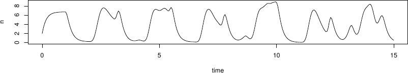
Here the solution of the model (to an accuracy of 1 part in ), took a quarter of a second.
5.1 Things can go wrong
The amazing combination of speed and accuracy apparent in many computer algorithms and numerical methods can lead to a false sense of security and the wrong impression that in translating mathematical and statistical ideas into computer code we can simply treat the numerical methods and algorithms we use as infallible ‘black boxes’. This is not the case, as the following three simple examples should illustrate. You may be able to figure out the cause of the problem in each case, but don’t worry if not: we will return to each of the examples in the course.
-
1.
The system.time function in R measures how long a particular operation takes to execute. First generate two matrices, and and a vector, .
Now form the product in two slightly different waysn <- 2000 A <- matrix(runif(n*n),n,n) B <- matrix(runif(n*n),n,n) y <- runif(n)
f0 and f1 are identical, to machine precision, so why is one calculation so much quicker than the other? Clearly anyone wanting to compute with matrices had better know the answer to this.system.time(f0 <- A%*%B%*%y)
##    user  system elapsed
##   0.838   0.040   0.227
system.time(f1 <- A%*%(B%*%y))
##    user  system elapsed
##   0.040   0.013   0.013
-
2.
It is not unusual to require derivatives of complicated functions, for example when estimating models. Such derivatives can be very tedious or difficult to calculate directly, but can be approximated quite easily by ‘finite differencing’. e.g. if is a function of then
where is a small interval. Taylor’s theorem implies that the right hand side tends to the left hand side, above, as . It is easy to try this out on an example where the answer is known, so consider differentiating w.r.t. .
The following plots the results. On the LHS is dashed, it’s true derivative is dotted and the FD derivative is continuous. The RHS shows the difference between the FD approximation and the truth.x <- seq(1,2*pi,length=1000) delta <- 1e-5 ## FD interval dsin.dx <- (sin(x+delta)-sin(x))/delta ## FD derivative error <- dsin.dx-cos(x) ## error in FD derivative
Note that the error appears to be of about the same magnitude as the finite difference interval . Perhaps we could reduce the error to around the machine precision by using a much smaller . Here is the equivalent of the previous plot, when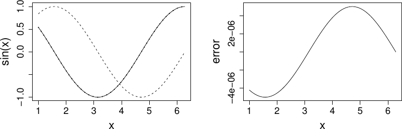
delta <- 1e-15
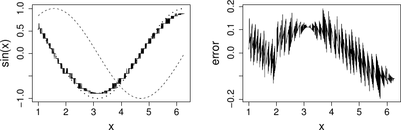
Clearly there is something wrong with the idea that decreasing must always increase accuracy here.
-
3.
These data
were generated with this code…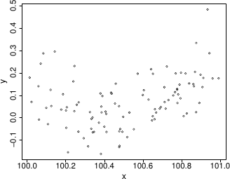 An appropriate and innocuous linear model for these data is , where the are independent, zero mean constant variance r.v.s and the are parameters. This can be fitted in R with
set.seed(1); n <- 100
xx <- sort(runif(n))
y <- .2*(xx-.5)+(xx-.5)^2 + rnorm(n)*.1
x <- xx+100
which results in the following fitted curve.b <- lm(y~x+I(x^2))
From basic statistical modelling courses, recall that the least squares parameter estimates for a linear model are given by where is the model matrix. An alternative to use of lm would be to use this expression for directly.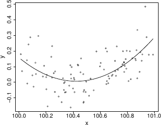 Something has gone badly wrong here, and this is a rather straightforward model. It’s important to understand what has happened before trying to write code to apply more sophisticated approaches to more complicated models.
X <- model.matrix(b) ## get same model matrix used above
## direct solution of ‘normal equations’
beta.hat <- solve(t(X)%*%X,t(X)%*%y)
## Error in solve.default(t(X) %*% X, t(X) %*% y): system is computationally singular: reciprocal condition number = 3.98647e-19
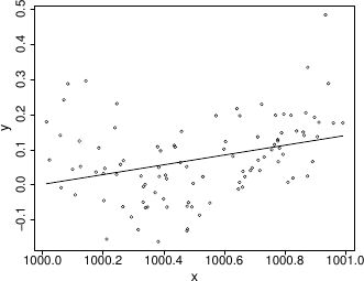
In case you are wondering, I can make lm fail to. Mathematically it is easy to show that the model fitted values should be unchanged if I simply add 900 to the x values, but if I refit the model to such shifted data using lm then the following fitted values result, which can not be correct.
6 Further reading
The course itself is supposed to provide an introduction to some numerical analysis that is useful in statistics, but if you can’t wait to get started than here is a list of some possibilities for finding out more.
-
Burden, R & J.D. Faires (2005) Numerical Analysis (8th ed) Brooks Cole. This is an undergraduate text covering some of the material in the course: the initial chapter is a good place to start for a discussion of computer arithmetic.
-
Press WH, SA Teukolsky, WT Vetterling and BP Flannery (2007) Numerical Recipes (3rd ed), Cambridge. This covers most of what we will cover in an easily digested form, but, as the name suggests, it is structured for those wanting to perform a particular numerical task, rather than for providing overview. The brief introduction to Error, Accuracy and Stability of numerical methods is well worth reading. (For random number generation the 3rd edition is a better bet than earlier ones).
-
Monahan, J.F. (2001) Numerical Methods of Statistics, Cambridge. This covers most of the course material and more, in a bit more depth than the previous books. Chapters 1 and 2 definitely provide useful background on good coding practice and the problems inherent in finite precision arithmetic. The rest of the book provides added depth on many of the other topics that the course will cover.
-
Lange, K. (2000) Numerical Analysis for Statisticians, Springer. This covers a more comprehensive set of material than the previous book, at a similar level, although with less discussion of the computational nitty-gritty.
If you want more depth still…
-
Golub, GH and CF Van Loan (1996) Matrix Computations 3rd ed. John Hopkins. This is the reference for numerical linear algebra, but not the easiest introduction.
-
Watkins, DS (2002) Fundamentals of Matrix Computations 2nd ed. Wiley. This is a more accessible book, but still aimed at those who really want to understand the material (for example, the author encourages you to write your own SVD routine, and with this book you can).
-
Nocedal and Wright (2006) Numerical Optimization 2nd ed. Springer, is a very clear and up to date text on optimization, which also covers automatic differentiation with great clarity.
-
Gill, P.E. , W. Murray and M.H. Wright (1981) Practical Optimization Academic Press, is a classic, particularly on constrained optimization. Chapter 2 is also an excellent introduction to computer arithmetic, numerical linear algebra and stability.
-
Ripley, B.D. (1987) Stochastic Simulation Wiley (re-published 2006). A classic on the subject. Chapters 2 and 3 are particularly relevant.
-
Cormen, T.H., C.E. Leiserson, R.L. Rivest and C. Stein (2001) Introduction to Algorithms (2nd ed.) MIT. Working with graphs, trees, complex data structures? Need to sort or search efficiently. This book covers algorithms for these sorts of problems (and a good deal more) in some depth.