Load up RStudio via your favourite method. If you can’t use RStudio for some reason, most of what we do in these labs can probably be done using WebR, but the instructions will assume RStudio. You will also want to have the web version of the lecture notes to refer to.
Ensure that you have all of the required R packages installed for the spatial part of the course.
Question 1
If you haven’t already done so, reproduce all of the plots and computations from Chapter 9 and Chapter 11 of the lecture notes by copying and pasting each code block in turn. Make sure you understand what each block is doing and that you can reproduce all of the plots.
Question 2
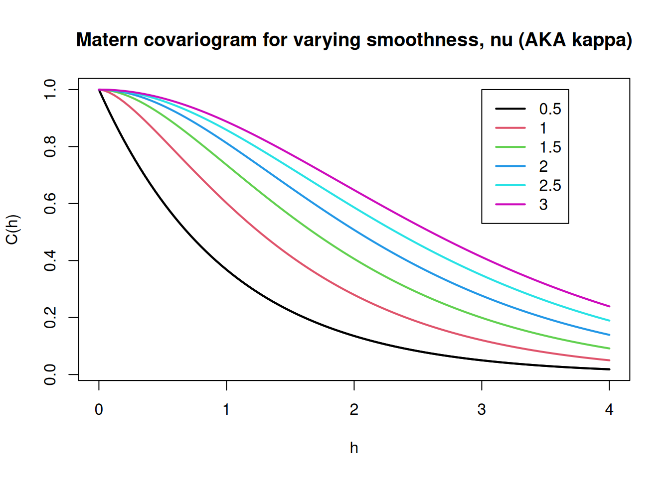
In the context of geostatistics, the Matérn covariance function is a very useful, flexible class of covariograms determining (weakly) stationary random fields with varying smoothness levels. At first sight it appears a little intimidating, due to the involvement of a Bessel function, but ultimately it is just a 3-parameter covariance function class, with a variance, scale, and roughness/smoothness parameter. The correlation function is available as a simple R function as geoR::matern (which in turn exploits base::besselK). We will use this function to get a better feel for the Matérn family.
Covariogram and semi-variogram
Let’s begin by plotting the covariogram for different values of the smoothing parameter, \(\nu\) (called kappa in geoR).
--------------------------------------------------------------
 Analysis of Geostatistical Data
 For an Introduction to geoR go to http://www.leg.ufpr.br/geoR
 geoR version 1.9-6 (built on 2025-08-29) is now loaded
--------------------------------------------------------------
The curve for \(\nu=0.5\) corresponds to the exponential covariogram, which is clearly not (twice) differentiable at \(h=0\). However, by the time we get to \(\nu=1\), the curve looks like it might be twice differentiable at 0. In fact, although we won’t prove it, the covariogram becomes twice differentiable at 0 for \(\nu>1\). This means that realisations of the process become differentiable iqm for \(\nu>1\). In fact, realisations become \(d\) times differentiable iqm (\(d\in\mathbb{N}\)) for all \(\nu>d\). So by using this class of covariance functions we have very fine-grained control on the level of smoothness that we expect in our realisations. This is one of many reasons for the popularity of the Matérn class.
Task A
Produce a plot similar to the one above, but for the semi-variogram rather than the covariogram.
Simulation
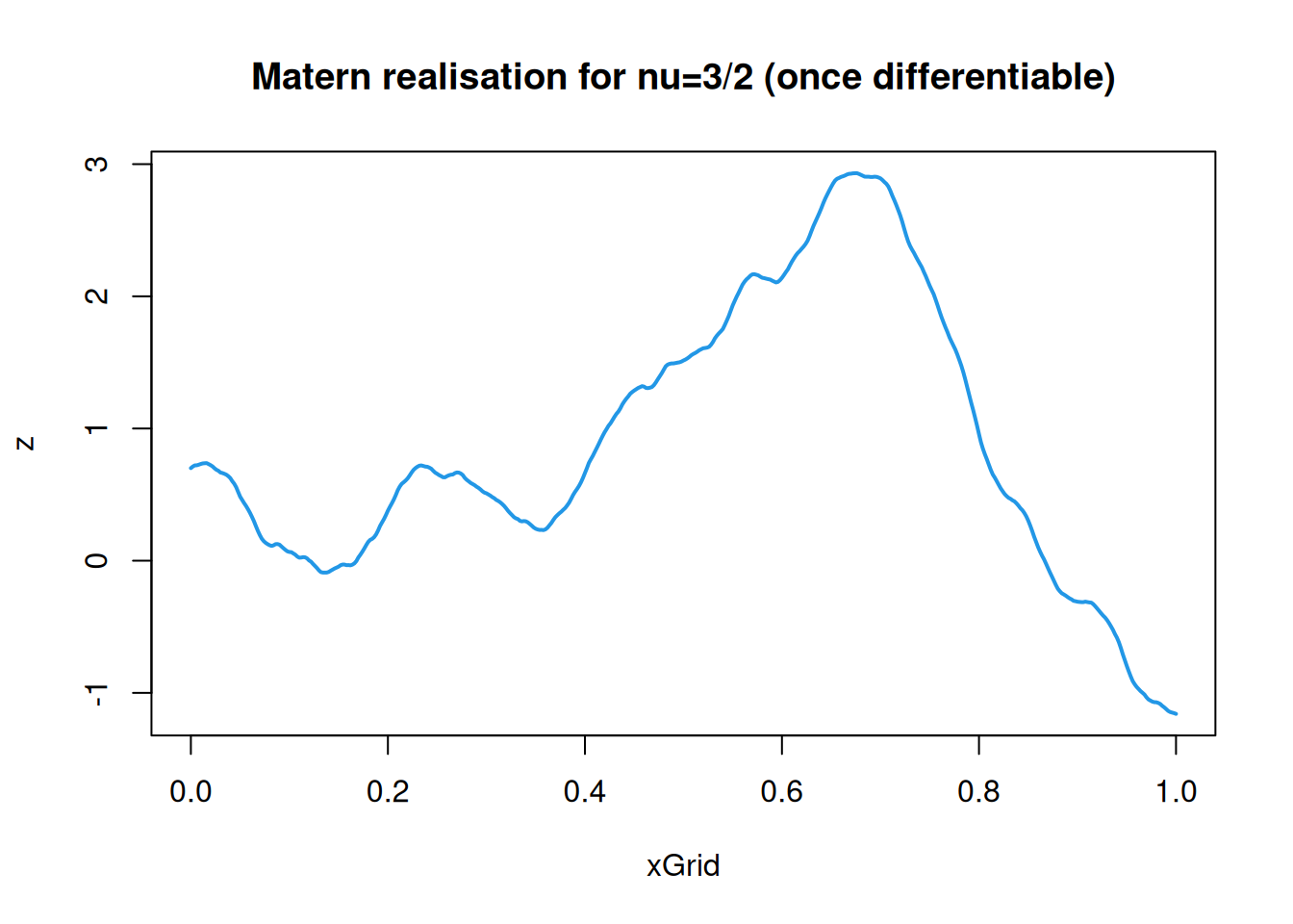
We can simulate realisations of the Matérn field using the covariance method discussed in Chapter 11. Below, a realisation for \(\nu=3/2\) (and \(\phi=1/10\)) is shown.
Produce a plot showing 5 independent realisations from this process.
Repeat for \(\nu=1/2\) (not differentiable) and \(\nu=5/2\) (twice differentiable).
Task C
On a 2-d grid of appropriate size, simulate a realisation of a 2-d Matérn field with \(\nu=3/2\).
Produce a selection of plots of this field. Try to create a nice plot.
Question 3 (optional)
Doing this question is optional, since it requires the registration of an API key with a service provider. But you should read through the question anyway. Read the following carefully before deciding how to proceed.
This question is concerned with overlaying spatial data on maps providing the spatial context. This can be done using the ggmap package, but this package downloads map tiles from map providers that require the registration of an API key. ggmap supports maps from Google and StadiaMaps. Both have a free tier for personal use, but Google requires credit card details to register, whereas StadiaMaps does not. For this question I suggest registering for an API key with StadiaMaps, and using it for plotting geostatistical data in context. Some people might not want to register for an API key simply because they don’t want to give their email address to a company they don’t know much about. Another reason you might not want to register for an API key right now is that when you first register with StadiaMaps you get a 14 day free trial of their professional tier. If you think this is something that you might want to take advantage of, then you might not want to waste your 14 day free trial now. But for most people, the free tier is fine, and there is no reason not to want to register an API key. You do not need to provide credit card details at any point in order to use the free tier.
First, if you don’t yet have it installed, install ggmap in the usual way: install.packages("ggmap"). Then load the package.
for some information about how to register your API key once you have one. Then go to StadiaMaps and follow their instructions to get a key. Create a “property” and copy the API key to your clipboard. Then register that key in R with a command like:
replacing the key with your personal key by pasting from the clipboard. Setting write=TRUE will write the key to your environment so that you don’t need to re-register it each time you start R. Your API key is personal to you: you should keep it secret. Once you have registered your API key, you should be ready to proceed.
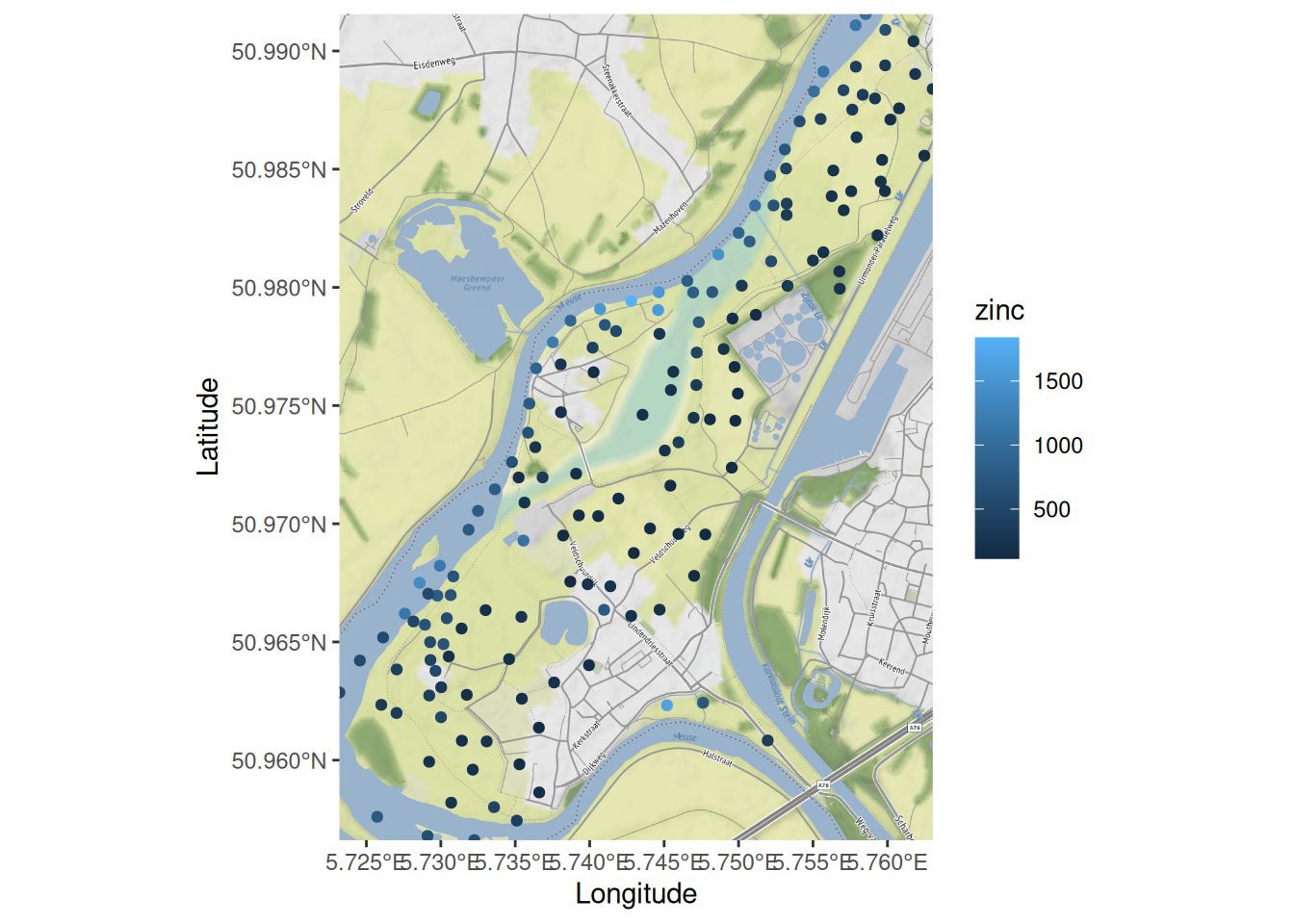
First, let’s load some more libraries and the Meuse data.
Next, let’s extract a bounding box for the dataset, and modify the names slightly for ggmap (ggmap likes the bounding box labelled slightly differently to sf, for some reason).
meuse_bb=st_bbox(meuse_sf2)# sf bbnames(meuse_bb)=c("left", "bottom", "right", "top")# ggmap-style bbmeuse_bb
    left   bottom    right      top
 5.72319 50.95661  5.76304 50.99156
Now we call on Stadia maps for a map tile corresponding to our bounding box.
Now we can see exactly why the data samples have been collected where they have.
It is incredibly useful and insightful to be able to view geostatistical data in context. Consult the ggmap documentation for further information about this package.
If you have completed all of the above, see if you can figure out how to use ggmap to plot a map of your home town. Investigate ways of customising the map. See ?get_stadiamap for details.