We now turn attention away from time series to spatial data. We will see that there are many similarities, but also some important differences. There a many different kinds of spatial data. Each kind may require a different modelling approach, and may be subject to different inferential questions. We will concentrate on the three or four most commonly encountered types of spatial data.
9.2 Point referenced data and geostatistics
Just as time series consist of observations indexed by time, spatial datasets typically consist of observations indexed by a point in space. So we can write \(z(\mathbf{s})\) for the value of an observation at location \(\mathbf{s}\). We will mainly consider univariate real-valued data, so then \(z(\mathbf{s})\in\mathcal{Z}\subset\mathbb{R}\), but multivariate extensions are possible. The spatial location belongs to the spatial domain, \(\mathcal{D}\), so \(\mathbf{s}\in \mathcal{D}\). This can typically be thought of as a point in 3-dimensional space, \(\mathcal{D}\subset \mathbb{R}^3\), but in practice most spatial data sets live in a two-dimensional sub-space, so we will typically have \(\mathcal{D}\subset\mathbb{R}^2\). We will also consider 1-d spatial data for illustrative purposes (and for linking back to time series models), so then \(\mathcal{D}\subset\mathbb{R}\). In this course we will assume that \(\mathcal{D}\) is a subset of a Euclidean vector space. However, this is a big assumption, since many spatial data sets are geospatial, and indexed by points on the surface of the Earth, which is most definitely not a Euclidean space! However, we will assume that the data sets that we are dealing with are over a sufficiently small area that projection onto \(\mathbb{R}^2\) is reasonable. A dataset consisting of \(n\) observations can typically be written \[
\{(\mathbf{s}_i, z(\mathbf{s}_i))\in \mathcal{D}\times\mathcal{Z}|i=1,2,\ldots,n\},
\] and the observed value \(z(\mathbf{s}_i)\) will often be written \(z_i\). In the context of geostatistics, the spatial locations are not considered to be random. They are typically irregularly distributed, but essentially arbitrary, and perhaps determined by the experimenter, either informally, or by some experimental design (which may be random, but the randomness in the design is not of inferential interest). It is the observations themselves that are typically considered to arise from some kind of random process. That is, the measurements \(z(\mathbf{s})\) are considered observations of the random variable \(Z(\mathbf{s})\), where \(\{Z(\mathbf{s})|\mathbf{s}\in\mathcal{D}\})\) is considered to be a random function (typically referred to as a random field or stochastic process) \(\mathcal{D}\rightarrow\mathcal{Z}\). The observations at different locations will typically not be iid (or exchangeable), since observations at nearby locations will typically be more highly correlated than observations at distant locations. In the context of geostatistics, this fact is often referred to as Tobler’s first law of geography: “everything is related to everything else, but near things are more related than distant things”.
The typical problem of inferential interest is interpolation (sometimes combined with smoothing), where data at the sites for which observations are available are used to make a prediction for the values that would be observed at sites for which measurements have not been made. That is, a prediction is wanted for \(Z(\mathbf{s})\), the unobserved value at an arbitrarily chosen site \(\mathbf{s}\in\mathcal{D}\), \(\mathbf{s}\notin\{\mathbf{s}_i|i=1,2,\ldots,n\}\).
9.2.1 The meuse dataset
There are many packages for working with spatial data in R. In the past, sp was the package used to define spatial datasets, and many packages built on top of this to add additional functionality. These days, sf (simple features) is the preferred base package for spatial data, and new packages for spatial analysis typically build on top of this. However, many useful packages still exist which rely on sp, so it is not possible to completely abandon this package yet. Recall that the CRAN spatial task view gives an invaluable summary of spatial packages in R. We will start by looking at a typical geostatistical dataset that is included in the sp package.
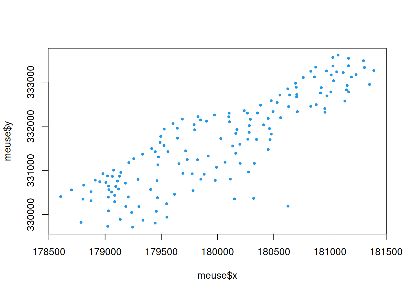
Use ?meuse to find out more about this data. We see that the first two columns of this data set give \(x\) and \(y\) coordinates of the spatial locations of the observervations, with respect to some coordinate system (discussed further below). There are then some columns representing some measurements, and some additional covariate information that we will ignore. We will focus mainly on the zinc column - a measurement of zinc concentration in the ground at each location. First, let’s just plot the spatial locations of the observations.
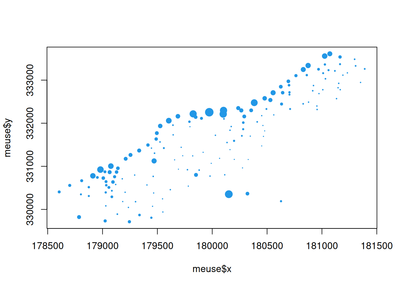
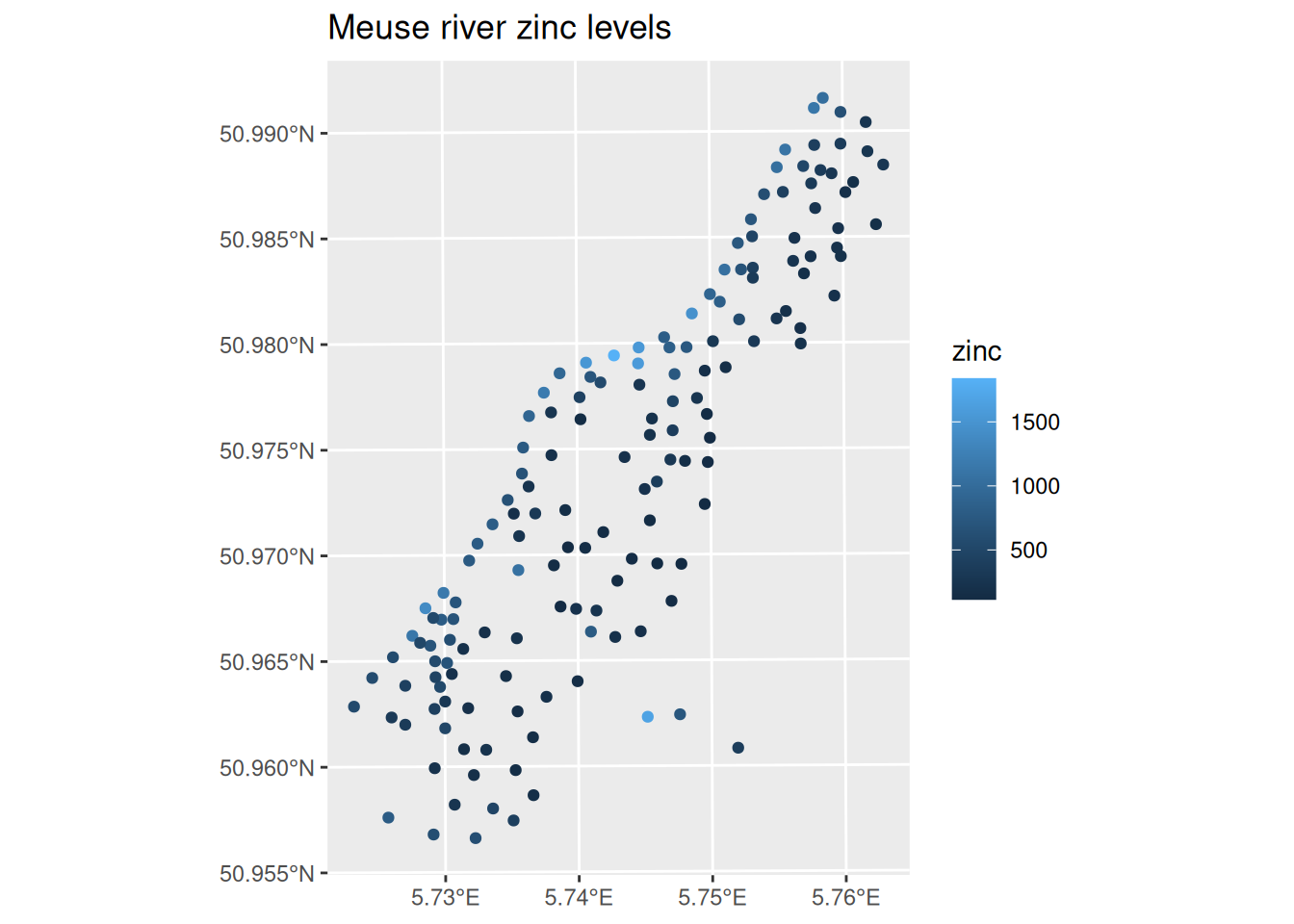
The measurements all lie to the east of the Meuse river (the Dutch side) next to the Dutch town of Stein, which is why there are no measurements in the top left of the plot. By looking at the range of zinc values, we can modify the plot to show levels of zinc concentration by the size of the plotted point.
We can now clearly see that zinc concentrations are typically higher close to the river, and lower further away, but with some variability.
Using the sf package, we can convert this data frame into an sf object. To do this, we will use the function st_as_sf. We will need to tell this function which columns contain the \(x\) and \(y\) coordinates, and also, what the coordinates mean (ie. what units they are in, and what they are measured with respect to). The help information (?meuse) confirms that the coordinates are RDH (a Dutch coordinate system). These have a coordinate reference system (CRS) code of EPSG:28992.
So meuse_sf is an object of class sf in addition to data.frame. We can plot objects of class sf.
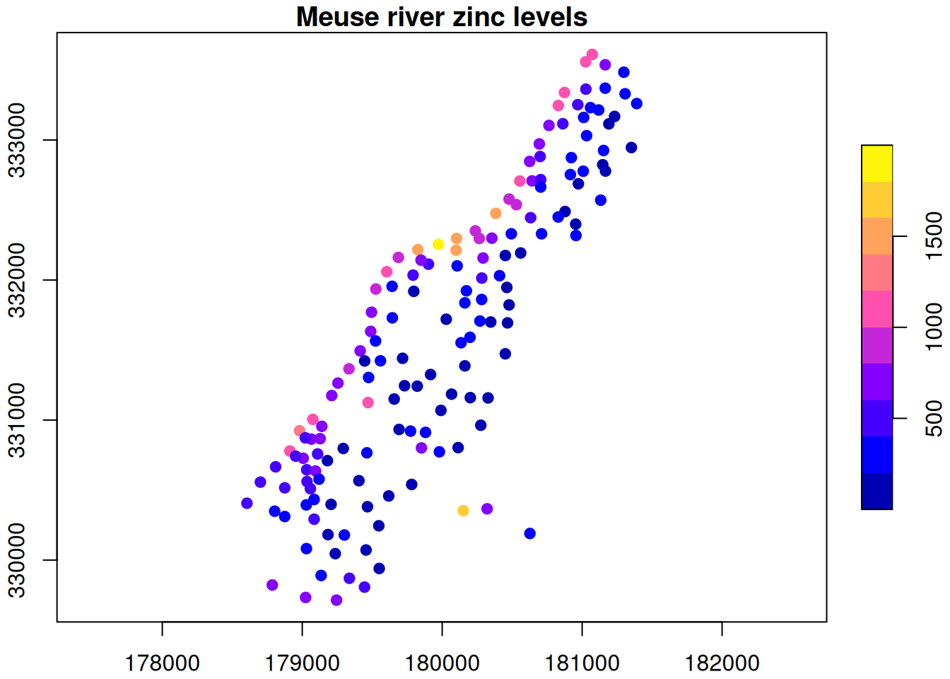
plot(meuse_sf[,"zinc"], pch=19,
     main="Meuse river zinc levels", axes=TRUE)
Here, a colour gradient is used to indicate zinc levels at each spatial location. In this course we will mainly use base R graphics, but sf objects work well with ggplot2 (and the tidyverse more generally).
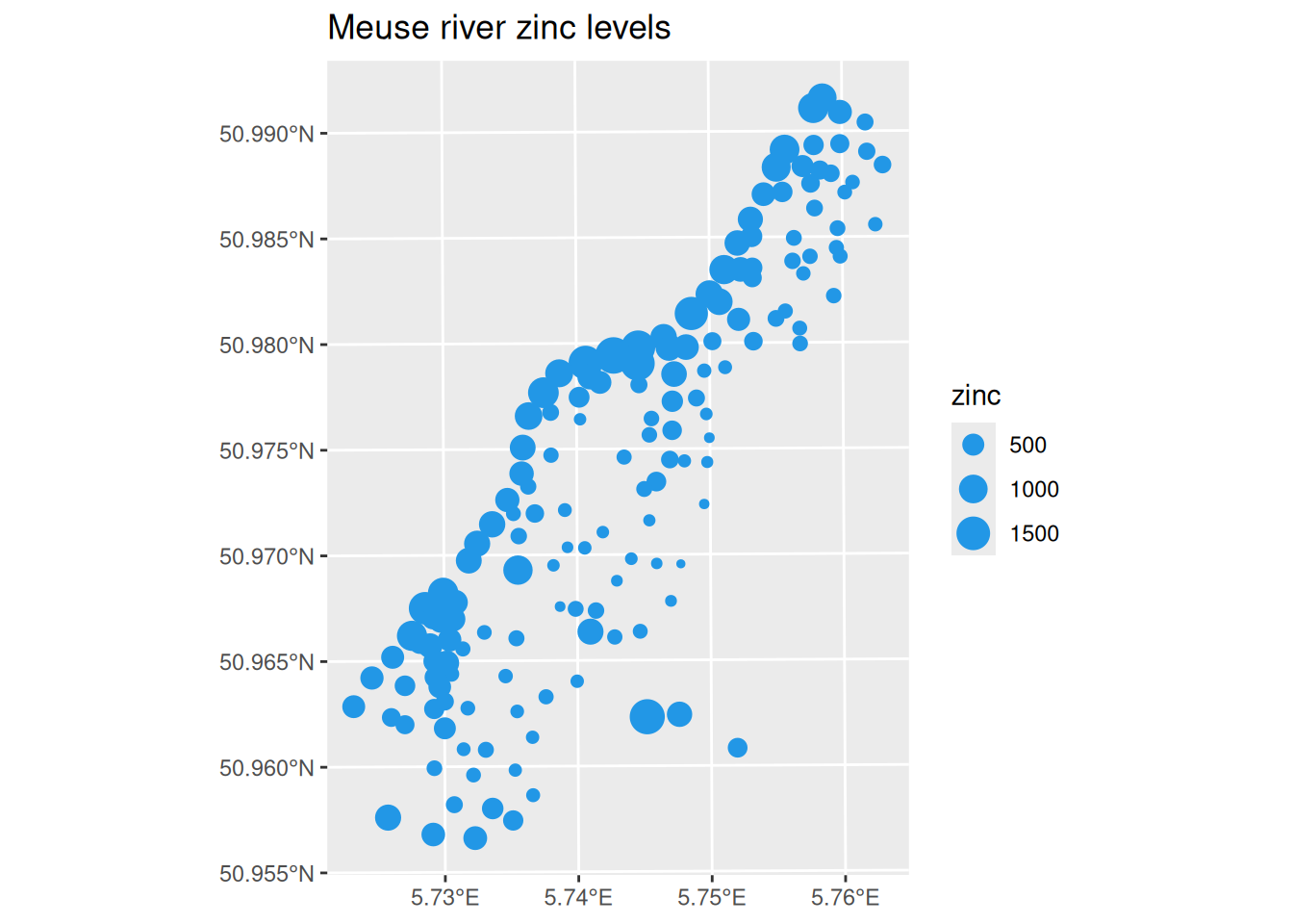
Note that the axes on the ggplot graphics show the spatial location in longitude and latitude. This is possible because the CRS allows mapping of coordinates to other coordinate systems. The function st_transform can be used to remap the coordinates in an sf object.
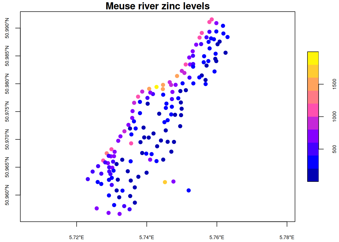
meuse_sf2=st_transform(meuse_sf, "EPSG:4326")plot(meuse_sf2[,"zinc"], pch=19, main="Meuse river zinc levels", axes=TRUE, cex.axis=0.6)
Note that 4326 is the EPSG code for WGS84, the current standard reference coordinate system for Earth (based on a 2-d longitude and latitude projection).
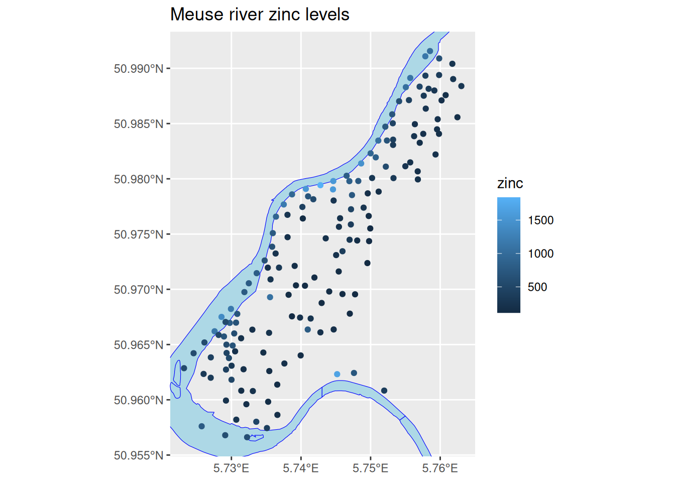
It would be helpful to see the data we have overlaid on a plot showing the course of the Meuse river. We can do that using the osmdata package to query OpenStreetMap data. Don’t worry about how this code works.
library(osmdata)meuse_bb=st_bbox(meuse_sf2)# bounding box in long/latmeuse_river=meuse_bb%>%opq()%>%add_osm_feature(key="water", value="river")%>%osmdata_sf()ggplot()+geom_sf(data =meuse_river$osm_polygons, colour ="blue", fill ="lightblue")+geom_sf(data =meuse_sf2, mapping=aes(colour=zinc))+coord_sf(xlim=c(meuse_bb[1], meuse_bb[3]), ylim=c(meuse_bb[2], meuse_bb[4]))+ggtitle("Meuse river zinc levels")
The standard statistical problem associated with data of this sort is to produce a smooth image containing a prediction of how the zinc levels vary across the entire spatial domain (possibly with some measure of uncertainty). The standard procedure for doing this is known as kriging.
9.3 Raster data and images
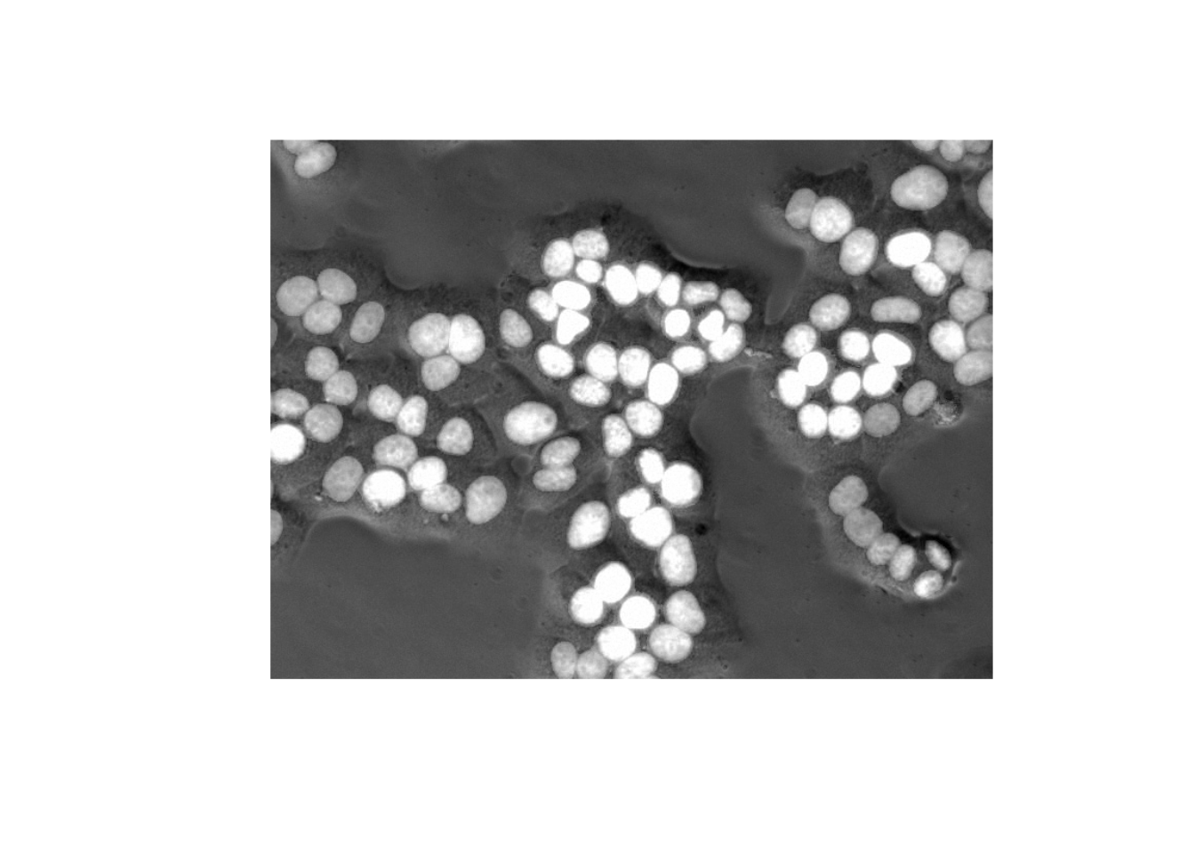
Raster data consist of data on a regular square grid, with each data location known as a pixel. Image data is of the same form. A basic (greyscale) image has a single real valued measurement at each pixel location. We could write this as \[
\{ z(\mathbf{s}_{i,j}) | i=1,2,\ldots,m,\ j=1,2,\ldots,n\}
\] Where now the sites are labelled by a row and column index. But in this case we will typically define \(z_{i,j}\equiv z(\mathbf{s}_{i,j})\), and will often consider these to be elements of the \(m\times n\) matrix \(\mathsf{Z}\).
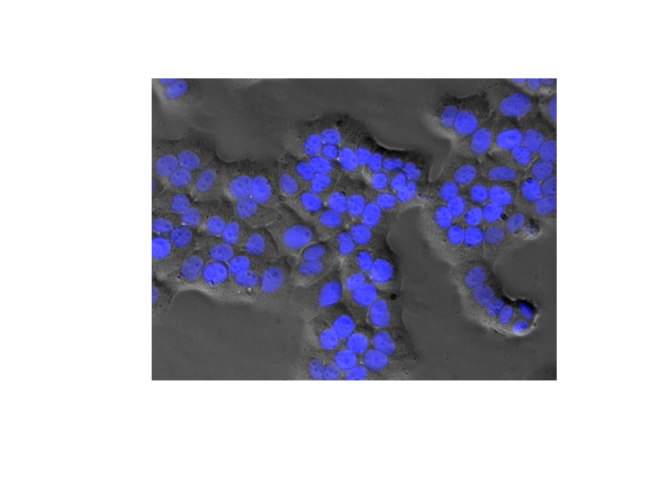
This gray image has a single real-valued intensity at each pixel location (the brighter the pixel, the higher the intensity). Here, the inferential problem is not interpolation, but typically smoothing/denoising, and sometimes segmentation.
9.3.2 Images as data on a regular square lattice
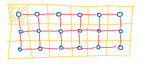
Image data can be thought of as data on a regular square lattice. Each node of the lattice represents a pixel, and the intensity of that pixel is associated with the corresponding node of the lattice. Nodes in the lattice have a natural neighbourhood structure, and can be joined by edges according to some simple criterion (eg. each node is joined to its four nearest neighbours). This neighbourhood structure can be used to define statistical models for images, induced by a corresponding model on the associated lattice/graph.
Image data as data on a square lattice
In the above figure, the yellow squares represent image pixels. The blue circles represent nodes of a graph, and the red lines denote edges joining the nodes of the lattice according to some neighbourhood structure. Here a first-order neighbourhood is used (4 nearest neighbours), but other neighbourhood structures are possible. Second order neighbourhood structures (8 nearest neighbours) are sometimes used, and these lead to statistical models with different properties.
First and second order neighbourhoods of a node on a 2d square lattice
9.4 Areal data and data on irregular lattices
Images are a very simple example of areal data. In an image, space is divided into squares called pixels, and the measurement or value associated with each pixel represents some kind of total or average or integral over that square region. Spatial data of this form is very common, but often space is not divided into a collection of identical squares.
When thinking about spatial data at large geographic scales, there are natural ways of segmenting space, corresponding to some kind of administrative unit. The Earth is divided into continents and continents are divided into countries. Countries are often divided into states. States are often divided into counties and counties are often divided into districts or parishes, etc. These units correspond to administrative areas, and it is natural to collect data aggregated at the level of these regions. However, these regions typically have complicated and irregular shapes.
Dealing with complex geographic data of this sort is the subject of geographic information systems (GIS). This is a huge topic which is not the main focus of this course. We will just learn about the bare minimum needed to do some interesting spatial analysis.
9.4.1 North Carolina SIDS dataset
For illustration, consider the US state of North Carolina (NC). The state is divided into 100 counties, and these are the main administrative units within the state. We can therefore think of NC as being the disjoint union of 100 areal regions. Administrative data is often collected at the county level. Here we will look at some health data, relating to the incidence of SIDS in NC. The data is in the spData package, and the spdep package is useful for building dependency structures between spatial regions.
Reading layer `sids' from data source
  `/home/darren/R/x86_64-pc-linux-gnu-library/4.5/spData/shapes/sids.gpkg'
  using driver `GPKG'
Simple feature collection with 100 features and 22 fields
Geometry type: MULTIPOLYGON
Dimension:     XY
Bounding box:  xmin: -84.32385 ymin: 33.88199 xmax: -75.45698 ymax: 36.58965
Geodetic CRS:  NAD27
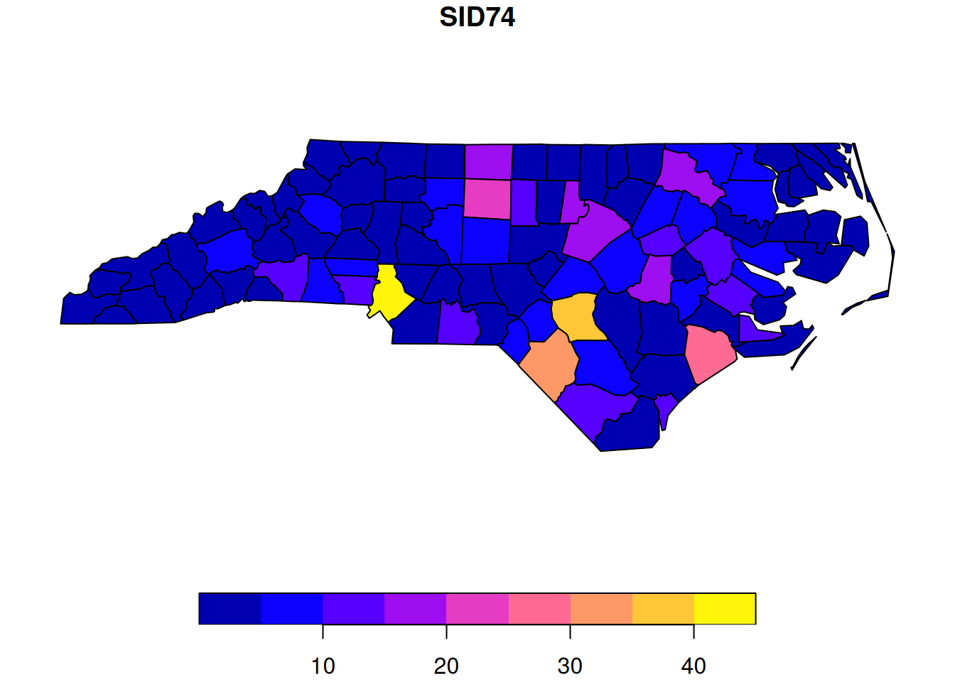
Here, we read the data from a GeoPackage file. This format is often used for storing complex geographic data in a standard way. This dataset contains many fields, but we will focus on the SID74 column.
This gives a nice visual representation of the data in its natural spatial context. We can see from the plot that nearby areas tend to be correlated, and so we would want any statistical models we use to take account the spatial context. In principle there are many ways that this could be done, but in practice, it is often done by mapping the data onto an irregular lattice, and defining appropriate statistical models on the lattice.
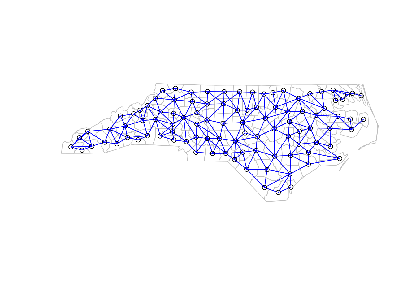
To map the areal problem to a lattice, we first need to define the nodes of the lattice. This is typically done by placing a node at the centroid of each region, but there are other possibilities. Then, some kind of neighbourhood structure is required to give the edges of the lattice. There are many possibilities here. One natural option is to join two regions by an edge if they share a common boundary. This is illustrated below (but don’t worry about what the code is doing).
Other options include joining regions to \(k\)-nearest neighbours, or joining regions if they are within a certain distance of one another. These different options will lead to models with different properties, and which is most appropriate will depend very much on the context. Some sort of weight will typically be associated with each edge, indicating the degree of relatedness of the two connected nodes. This could be a function of the distance between the nodes, but there are other possibilities.
9.5 Spatial point data
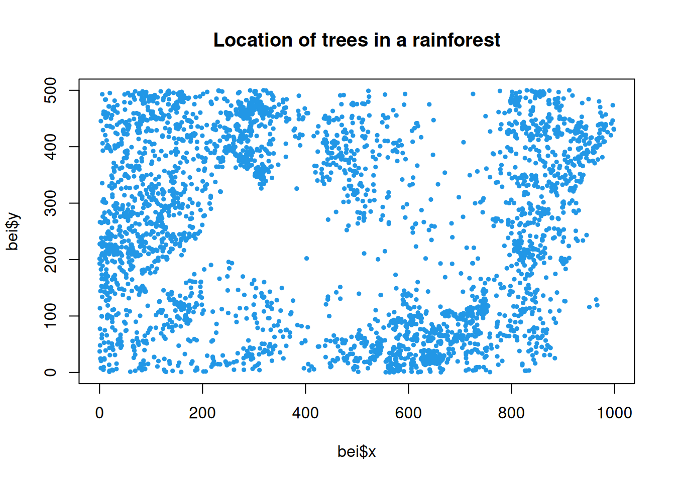
The final kind of spatial data that we will consider in this course is spatial point pattern data, for data arising from some kind of spatial point process. Here it is the locations of the data points that are of interest. It is the spatial locations that are measured, and considered random. They are not chosen by the experimenter. The location of trees in a natural rainforest would be a good example of spatial point data. The spatstat package is useful for the analysis of spatial point data, and contains some example datasets.
Planar point pattern: 3604 points
window: rectangle = [0, 1000] x [0, 500] metres
plot(bei$x, bei$y, pch=19, cex=0.5, col=4,
     main="Location of trees in a rainforest")
We can clearly see that the tree locations are not uniformly distributed within the sampling window. There are distinct areas where there are very few trees, and other areas where trees are densely packed. We would say that the trees are clustered in a non-uniform way. Assessing whether points are uniformly distributed, and if not, how they deviate from uniformity, is a typical inferential question in spatial point data analysis.
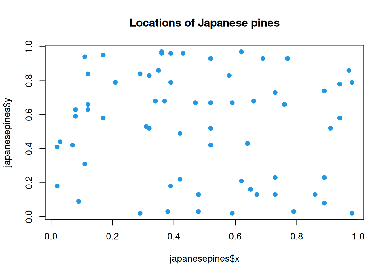
In contrast, below are the locations of some Japanese Pines.
plot(japanesepines$x, japanesepines$y, pch=19, col=4,
     main="Locations of Japanese pines")
This distribution looks as though it could be uniformly randomly distributed. It is not that the trees are perfectly evenly spread. There are examples of pairs of trees that are very close together, and trees that are far from other trees. But these are things that one would expect to arise by chance, even if the true data generating mechanism is uniformly random.
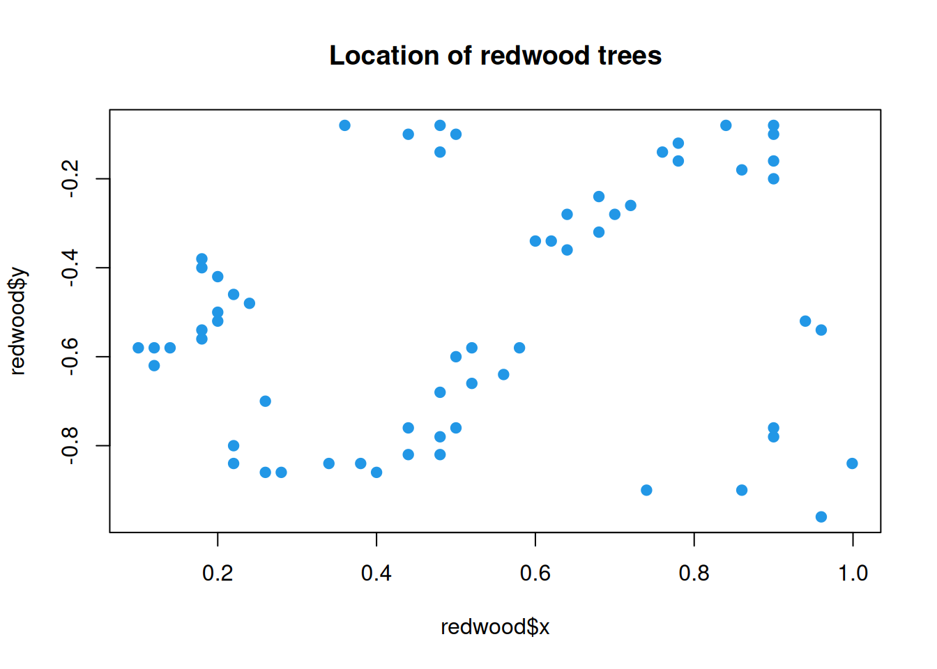
Below is another example of tree locations that are clustered.
plot(redwood$x, redwood$y, pch=19, col=4,
     main="Location of redwood trees")
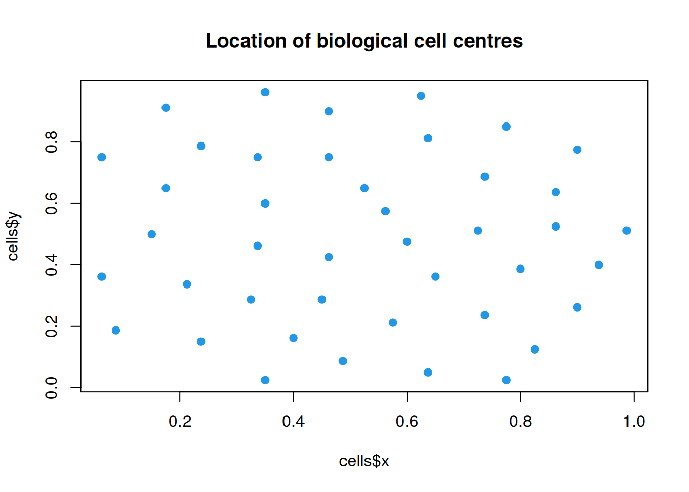
But not all deviations from uniformity are clusterings. Below is some data showing the locations of the centres of some biological cells under a microscope.
plot(cells$x, cells$y, pch=19, col=4,
     main="Location of biological cell centres")
We see that these points are very evenly spread - too evenly to have arisen by chance from a uniformly random process. There are no pairs of points that are very close (and no points that are exceptionally far away from all other points). Here there is a repulsive mechanism that is keeping the cell centres from getting too close to one another. This deviation from randomness is in some ways the opposite of the clustering we have observed in other point pattern examples. Detecting this kind of repulsive mechanism is also of inferential interest.
9.5.1 Marked point patterns
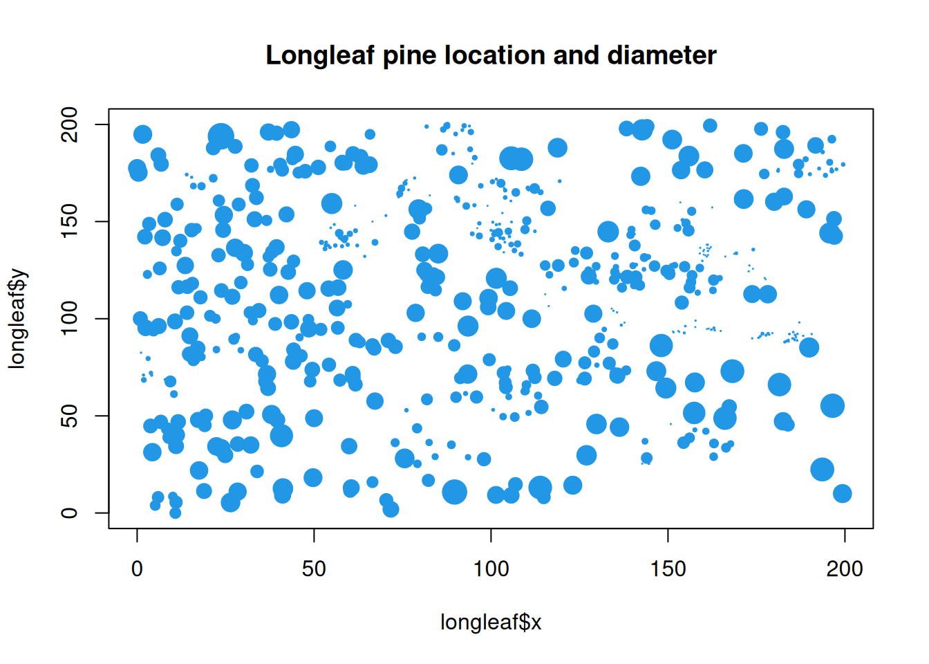
Sometimes there are measurements associated with each point, in addition to its location. Such data is called a marked point pattern. A random mechanism generating such data is called a marked point process. For example, in the context of trees, in addition to measuring the location of each tree, one could also measure the tree diameter.
plot(longleaf$x, longleaf$y, cex=longleaf$marks/30, pch=19, col=4,
     main="Longleaf pine location and diameter")
Understanding whether there is any relationship between the marking and the (relative) position of the point is a typical inferential question.
9.6 Fully spatio-temporal data
At the end of the course we will put together what we know about time series with what we know about spatial statistics in order to try and make sense of fully spatio-temporal data - that is, data associated with both a point in space and a specific time. Again, there are many different kinds of spatio-temporal data, each requiring a different modelling approach. We will concentrate on classical geostatistical spatio-temporal data, consisting of a collection of time series from some fixed but irregularly located sites. We can then write our observations as \(z(\mathbf{s}_i, t)\). A typical example might be recordings of daily maximum temperature at a fixed collection of spatially distributed weather stations over a common time window. We will defer further discussion of spatio-temporal data and modelling until the final chapter.
