A Gaussian process (GP) is a second-order random field whose finite-dimensional distributions are all jointly multivariate Gaussian. Since a multivariate Gaussian random quantity is completely determined by its mean vector and covariance matrix, and since the mean and covariance function of a second-order random field completely determines the mean vector and covariance matrix of any finite collection of sites, a GP is completely determined by its mean, \(\mu(\cdot)\) and covariance function, \(C(\cdot,\cdot)\). So, for any finite collection of sites \(\mathbf{s}_1,\mathbf{s}_2,\ldots,\mathbf{s}_n\in\mathcal{D}\subset\mathbb{R}^d\), we can construct mean vector, \[
\pmb{\mu} = [\mu(\mathbf{s}_1),\mu(\mathbf{s}_2),\ldots,\mu(\mathbf{s}_n)]^\top,
\] and covariance matrix, \[
\mathsf{C} = \begin{pmatrix}
C(\mathbf{s}_1,\mathbf{s}_1) & C(\mathbf{s}_1,\mathbf{s}_2) & \cdots & C(\mathbf{s}_1,\mathbf{s}_n) \\
C(\mathbf{s}_2,\mathbf{s}_1) & C(\mathbf{s}_2,\mathbf{s}_2) & \cdots & C(\mathbf{s}_2,\mathbf{s}_n) \\
\vdots & \vdots & \ddots & \vdots \\
C(\mathbf{s}_n,\mathbf{s}_1) & C(\mathbf{s}_n,\mathbf{s}_2) & \cdots & C(\mathbf{s}_n,\mathbf{s}_n) \\
\end{pmatrix},
\] to get \[
\mathbf{Z}\equiv [Z(\mathbf{s}_1),Z(\mathbf{s}_2),\ldots,Z(\mathbf{s}_n)]^\top\sim \mathcal{N}(\pmb{\mu}, \mathsf{C}).
\]
We call a GP stationary if it is additionally a weakly stationary random field. In this case the GP is completely determined by its mean \(\mu\in\mathbb{R}\) and covariogram function, \(C(\cdot):\mathcal{D}\rightarrow\mathbb{R}\). Note that since a GP is completely determined by its first two moments, if it is weakly stationary, it will also be strictly stationary, and there will be no need to distinguish the two cases. Similarly, a GP is intrinsically stationary if it is additionally an intrinsically stationary random field. Note that if we fix an intrinsically stationary GP at a given spatial location (such as the origin), then its distribution will be completely determined by the (semi-)variogram function, \(\gamma(\cdot):\mathcal{D}\rightarrow\mathbb{R}\).
11.2 Simulation
Since GPs have fully determined joint probability distributions (given a mean and covariance function), we can (in principle, at least), simulate exact realisations of the process (on a computer). Stochastic simulation is a very powerful technique in probability and statistics, so we will investigate this in detail. We obviously can’t work directly with infinite-dimensional random quantities, but so long as we always work with finite-dimensional projections, everything works out fine. If we want to get a feel for what a GP “looks like”, we can simulate it on a finite regular grid/lattice of spatial locations.
To illustrate the basic idea, we will simulate a simple stationary GP with zero mean and (squared-exponential) covariogram \[
C(\mathbf{h}) = \exp\{-64\Vert\mathbf{h}\Vert^2\},
\] which has a length scale of \(1/8\).
11.2.1 Simulating GPs on a 1d grid
In 1d we can just take a collection of equispaced points along the real line, and then create a matrix of pairwise distances between them (using the dist function) in order to construct a covariance matrix.
set.seed(42)# fix a seed for reproducibilityxGrid=seq(0, 1, 0.002)# regular grid of x valueslength(xGrid)
[1] 501
hMat=as.matrix(dist(xGrid))# matrix of pairwise Euclidean distancesdim(hMat)
[1] 501 501
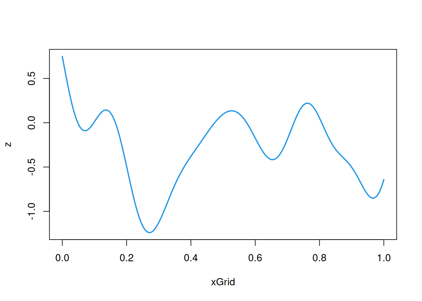
cf=function(h)exp(-64*h^2)# covariance/covariogram functionz=mvtnorm::rmvnorm(1, sigma=cf(hMat))# single sample from a MVNplot(xGrid, z, type='l', col=4, lwd=2)# plot the realisation
We see that the realisation based on the squared-exponential covariance is a very smooth random function. Of course, we shouldn’t just look at one realisation.
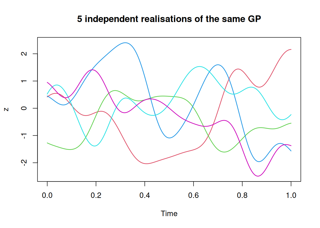
z=mvtnorm::rmvnorm(5, sigma=cf(hMat))# 5 independent samples from a MVNplot(ts(t(z), start=0, deltat=0.002), plot.type="single", col=2:6, lwd=1.5, ylab="z", main="5 independent realisations of the same GP")
This strategy works well, but comes with a significant computational cost. If we want to simulate a realisation on \(n\) grid points, then we need to construct an \(n\times n\) covariance matrix, which has storage requirements that are \(\mathcal{O}(n^2)\), but then simulation will require the formation of some kind of square root of the covariance matrix, which will have a computational cost that is \(\mathcal{O}(n^3)\). We can just about tolerate this for simulation in 1d, but this becomes a genuine constraint for 2d simulation.
11.2.2 Simulating GPs on a 2d grid
In 2d things are very slightly more complicated. We want to construct a regular grid/lattice of points in 2d to see how the process behaves on this grid of points. A reasonably coarse grid should be used in order to avoid the construction and decomposition of huge covariance matrices. We can use the function expand.grid to create the relevant combinations of \(x\) and \(y\) values, and then again use the dist function to create a matrix of pairwise Euclidean distances between the points. Once we have a realisation from the correct MVN distribution, we can turn that vector into a matrix for plotting.
xGrid=seq(0, 1, 0.02)# coarser grid (since dimension will be squared)length(xGrid)
[1] 51
xyGrid=expand.grid(xGrid, xGrid)# regular grid of x-y valuesdim(xyGrid)
[1] 2601 2
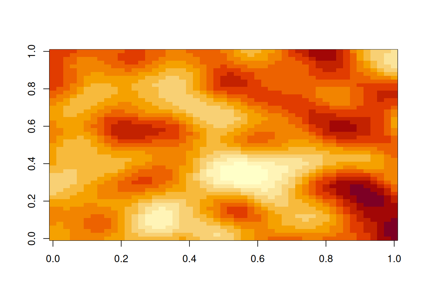
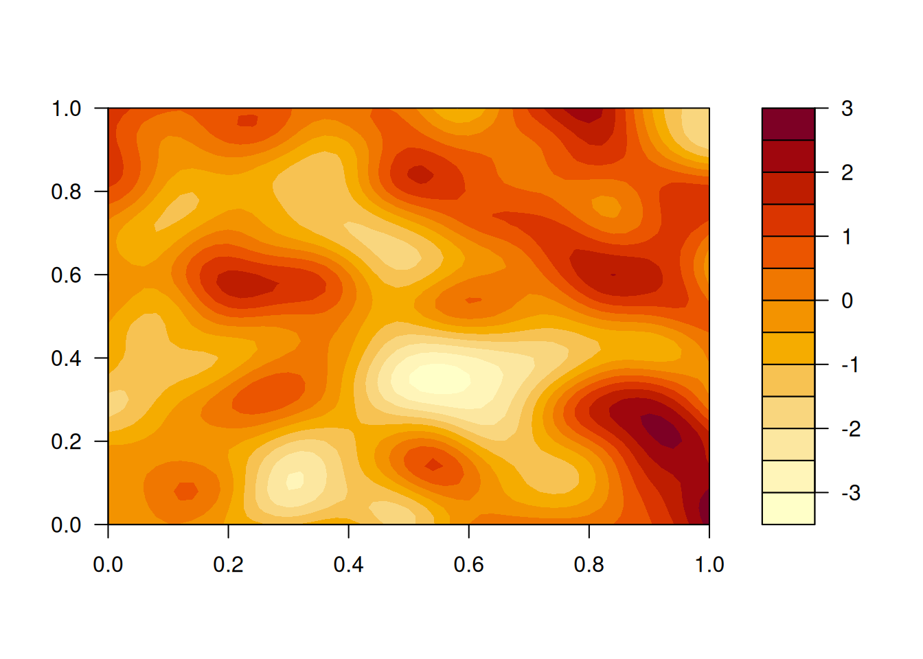
hMat=as.matrix(dist(xyGrid))# matrix of pairwise Euclidean distancescf=function(h)exp(-64*h^2)# covariogram function (as a function of distance)zVec=mvtnorm::rmvnorm(1, sigma=cf(hMat))# single sample from a MVNz=matrix(zVec, nrow=length(xGrid))# wrap vector into a matriximage(z)# plot the matrix as a colour image
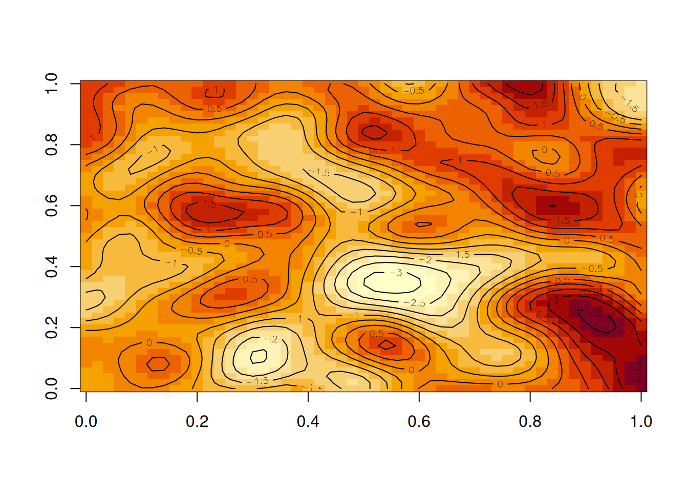
If we want, we can overlay contours on top of the image. Alternatively, we can use the filled.contour function, which works well for smooth GPs, but less well for GPs with rough realisations.
image(z)# plot the matrix as a colour imagecontour(z, add=TRUE)# overlay contours if desired
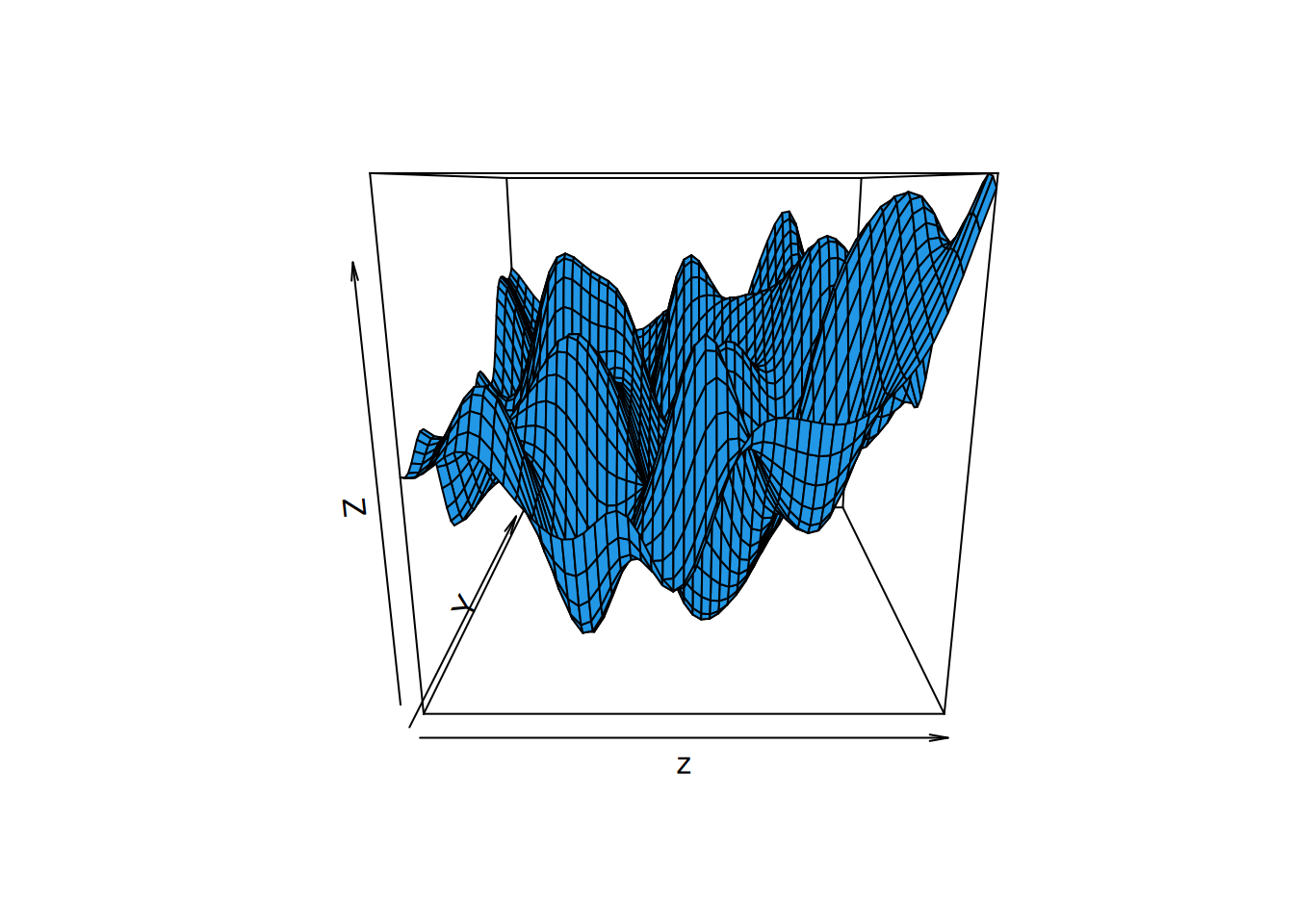
persp(z, col=4)# alternatively, a 3d perspective plot can be made
Alternatively, we can construct 3d perspective plots.
11.3 Example GPs
11.3.1 Squared-exponential covariogram
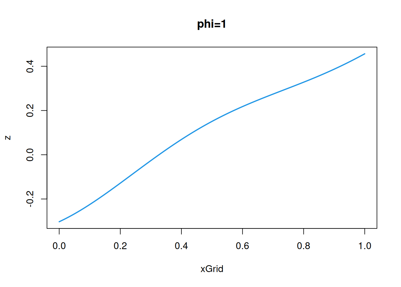
Let’s look more at a stationary GP with a squared-exponential covariogram. This is often used in applications where the underlying random field being modelled is thought to vary in a very smooth way. \[
C(\mathbf{h}) = \sigma^2\exp\{-(\Vert\mathbf{h}\Vert/\phi)^2\},\quad \mathbf{h}\in\mathcal{D}.
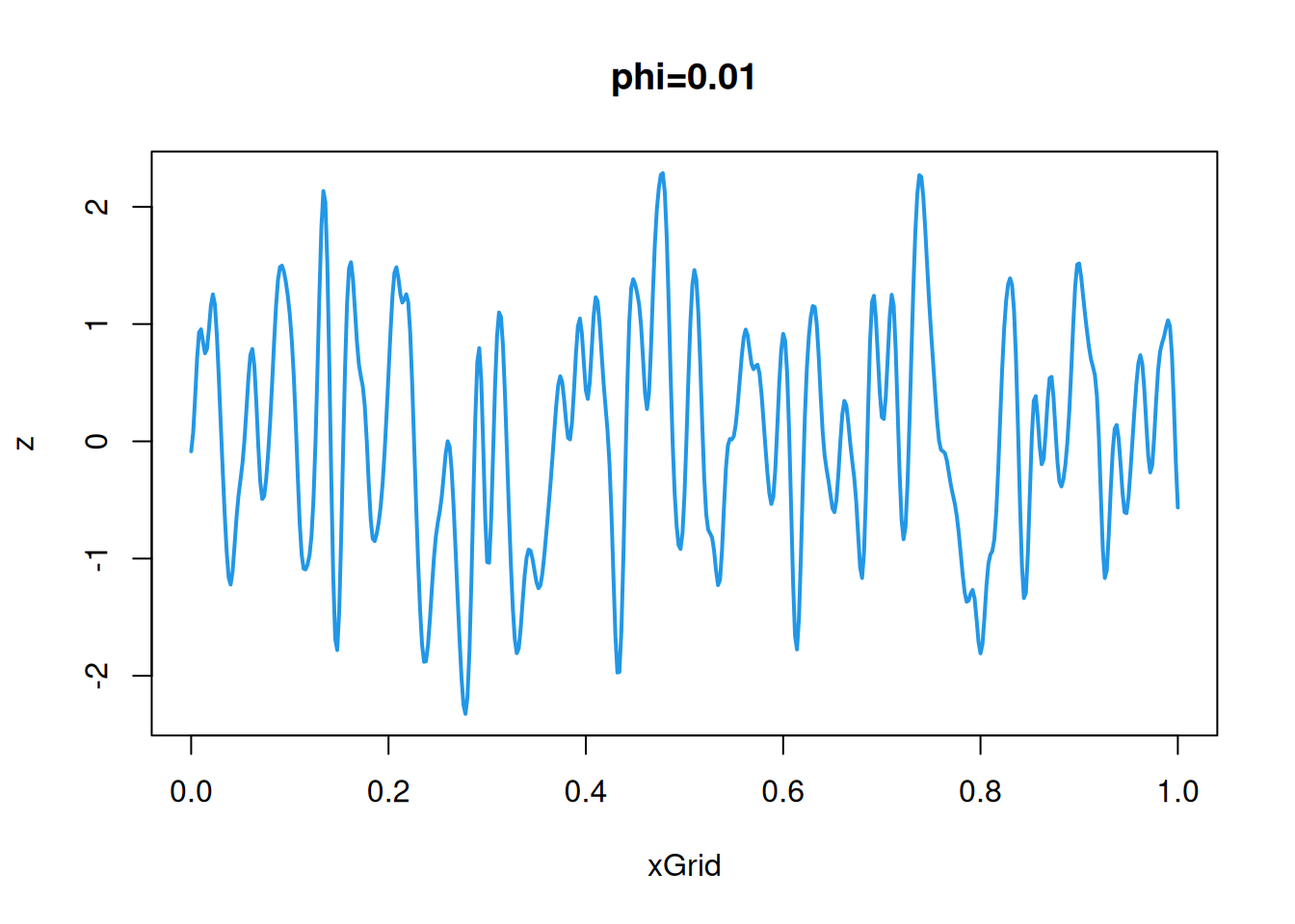
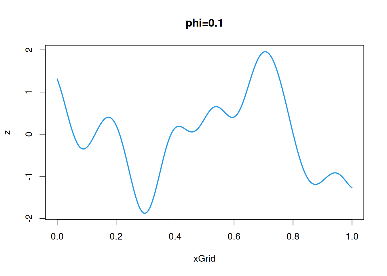
\] We use the typical parameterisation, in terms of stationary variance, \(\sigma^2\), and length scale \(\phi\). The two parameters have a very simple interpretation. Increasing the parameter \(\sigma\) stretches the process vertically, and the increasing the parameter \(\phi\) stretches the process horizontally. The stationary variance is fairly intuitive, so let’s just fix that to \(\sigma=1\) and look at varying the length scale, \(\phi\), in the simpler 1d case.
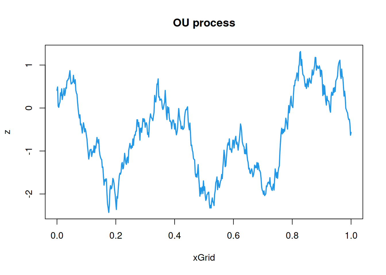
Since the OU process has the Markov property, the smart way to simulate realisations from this process (at least in 1d) is to sequentially sample from the transition kernel of the process. However, we will ignore this and use its covariance function to sample, as we would for processes without the Markov property. \[
C(\mathbf{h}) = \sigma^2\exp\{-\Vert\mathbf{h}\Vert/\phi\},\quad \mathbf{h}\in\mathcal{D}.
\] The parameters of this process behave similarly to the corresponding parameters in the squared exponential covariance function, so we will just fix them at \(\sigma=1\), \(\phi=0.2\) for the purposes of simulation. Again, we start with the 1d case.
This sample path is consistent with that we simulated in Chapter 2, but it is qualitatively different to the sample paths associated with a squared-exponential covariogram. Clearly we should be cautious about making strong statements regarding sample path regularity from a collection of values on a finite grid, and we will see how to approach this problem analytically in Section 11.4. Nevertheless, it looks as though the sample paths associated with a squared-exponential covariogram are both continuous and differentiable, whereas the sample paths associated with the OU process are continuous but nowhere differentiable. This turns out to be true, so the sample paths associated with the squared-exponential covariogram are smooth, whereas those associated with the exponential covariogram are rough, and hence there is a qualitative difference in the regularity of sample paths associated with these two very similar looking covariograms.
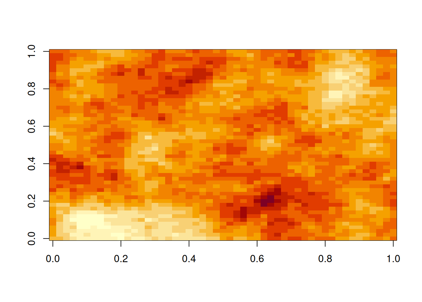
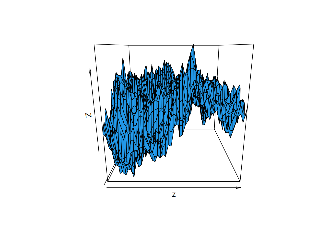
We can also sample surfaces in 2d.
xGrid=seq(0, 1, 0.02)# coarser grid (since dimension will be squared)xyGrid=expand.grid(xGrid, xGrid)hMat=as.matrix(dist(xyGrid))zVec=mvtnorm::rmvnorm(1, sigma=cf(hMat))z=matrix(zVec, nrow=length(xGrid))image(z)
Again, we should be cautious due to the coarseness of the grid, but this surface appears to be continuous but not differentiable. It is therefore rough, whereas the surface associated with a squared-exponential covariogram is smooth.
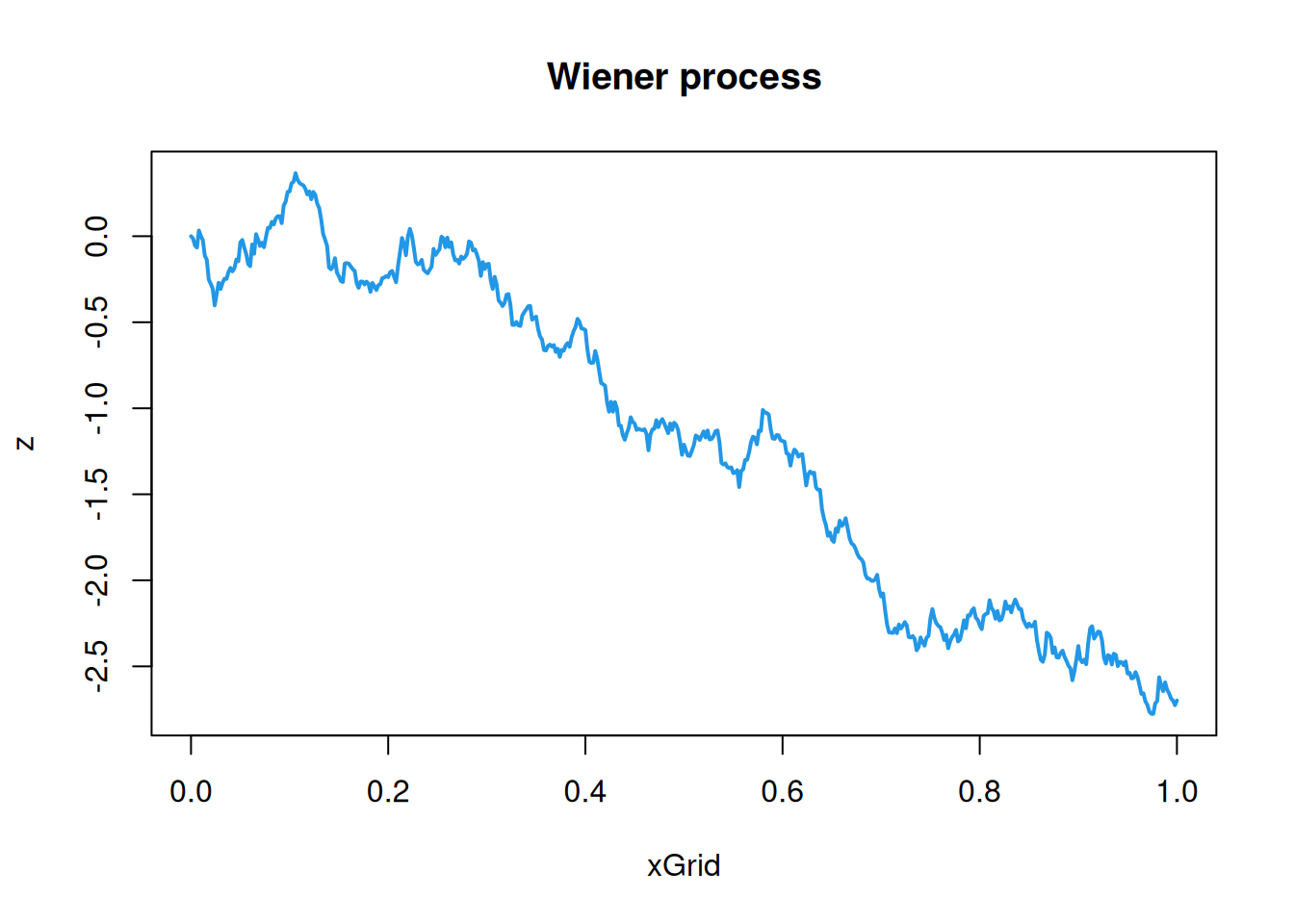
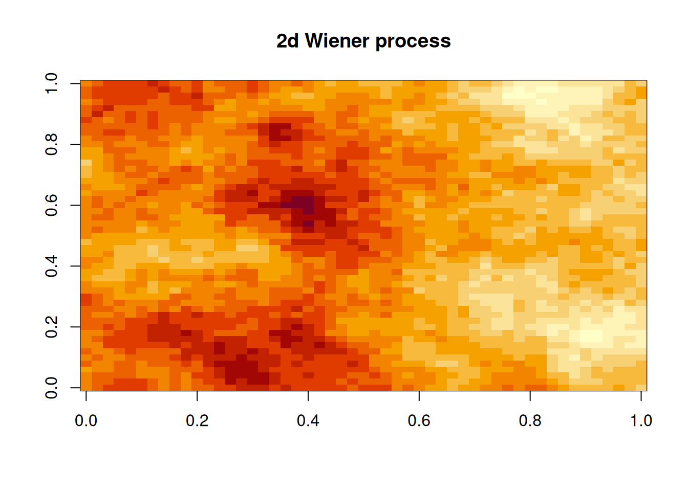
11.3.3 Wiener process
Again, the Wiener process has the Markov property, and this can be exploited for simulation. However, we will ignore this and sample directly from the covariance function, since we will need to do that for fBM (which is not Markovian, in general) anyway. The Wiener process is intrinsically stationary, but not stationary, so we will have to adapt our simulation strategy to this case, using a covariance function with two arguments, \[
C(\mathbf{s},\mathbf{s}') = \frac{1}{2}\left( \Vert\mathbf{s}\Vert + \Vert\mathbf{s}'\Vert - \Vert\mathbf{s}-\mathbf{s}'\Vert \right),\quad \mathbf{s},\mathbf{s}'\in\mathcal{D}.
\] We begin with the 1d case.
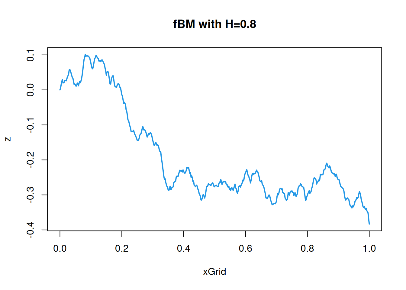
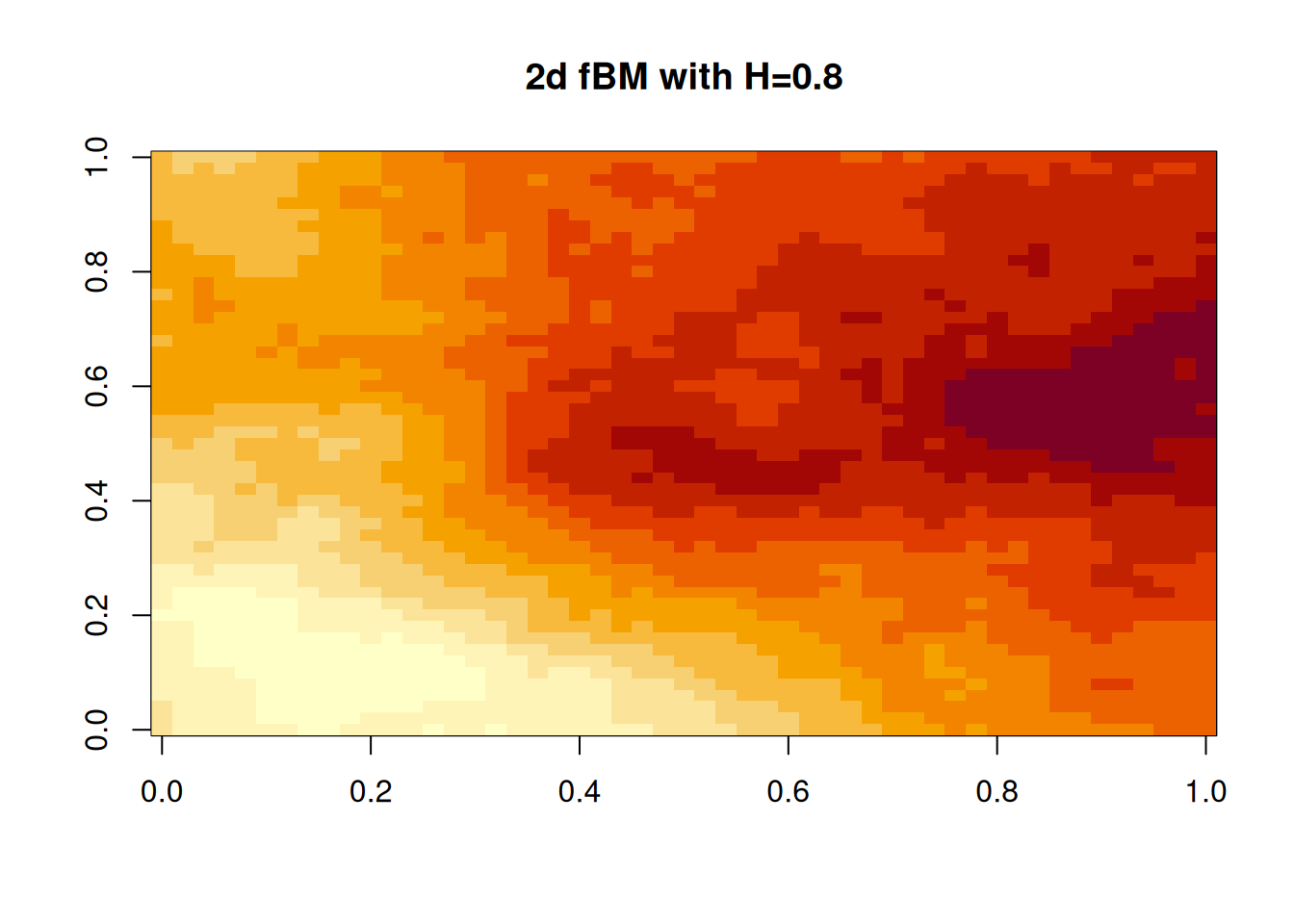
The approach we have used for the Wiener process adapts trivially to fBM with covariance function \[
C(\mathbf{s},\mathbf{s}') = \frac{1}{2}\left( \Vert\mathbf{s}\Vert^{2H} + \Vert\mathbf{s}'\Vert^{2H} - \Vert\mathbf{s}-\mathbf{s}'\Vert^{2H} \right),\quad \mathbf{s},\mathbf{s}'\in\mathcal{D}.
\] We will generate samples using \(H=0.8\), since this is often felt to correspond to the smoothness of many processes observed in nature. 1d first.
These fBM paths and surfaces for \(H=0.8\) look smoother than Wiener process but rougher than those of a GP with a squared-exponential covariance function.
11.4 Regularity (continuity and differentiability)
The sample paths from a GP with a squared exponential covariogram seem very “smooth”, whereas the sample paths of an OU process seem rather “rough”. Can we say anything precise about the regularity of GP sample paths?
11.4.1 Continuity
Let’s start by thinking about the continuity of sample paths. Many of the examples we have looked at seem to have continuous sample paths, but it also seems intuitively obvious that a nugget process will not, so we cannot assume that all GPs have continuous sample paths. We know from analysis how to define the continuity of a function at a given point, but here care is required in the interpretation of this definition, due to the randomness of the process. We want to say that \(Z(\mathbf{s})\) is continuous at \(\mathbf{s}\) if “\(Z(\mathbf{s}+\mathbf{h}) \overset{\mathbf{h}}{\underset{\mathbf{0}}{\longrightarrow}} Z(\mathbf{s})\)” in some appropriate sense, or equivalently, “\(Z(\mathbf{s}+\mathbf{h}) - Z(\mathbf{s}) \overset{\mathbf{h}}{\underset{\mathbf{0}}{\longrightarrow}} 0\)”, since now only the LHS is random.
There are many different senses in which a random quantity can tend to zero. Here we focus on convergence in quadratic mean, so we say that the random quantity \(X(\mathbf{h})\) tends to zero in quadratic mean (iqm) if \(\mathbb{E}[X(\mathbf{h})^2]\) tends to zero as \(\mathbf{h}\) tends to zero. Note that this implies that both the expectation and variance of the random quantity must tend to zero, so this is quite a powerful notion of convergence in general, and even more so in the case of Gaussian random quantities, which we are primarily concerned with here.
Returning to our original problem, we say that a process is continuous iqm at \(\mathbf{s}\) if \[
Z(\mathbf{s}+\mathbf{h}) - Z(\mathbf{s}) \overset{\mathbf{h}}{\underset{\mathbf{0}}{\longrightarrow}} 0, \quad \text{iqm},
\] or equivalently, \[
\mathbb{E}\left[\left\{ Z(\mathbf{s}+\mathbf{h}) - Z(\mathbf{s}) \right\}^2\right] \overset{\mathbf{h}}{\underset{\mathbf{0}}{\longrightarrow}} 0.
\] For an intrinsically stationary random field with semi-variogram \(\gamma(\cdot)\), we have \[\begin{align*}
\mathbb{E}\left[\left\{ Z(\mathbf{s}+\mathbf{h}) - Z(\mathbf{s}) \right\}^2\right] &= \left\{\mathbb{E}\left[ Z(\mathbf{s}+\mathbf{h}) - Z(\mathbf{s})\right]\right\}^2 + \mathbb{V}\mathrm{ar}\left[Z(\mathbf{s}+\mathbf{h}) - Z(\mathbf{s})\right] \\
&= (\mu - \mu)^2 + 2\gamma(\mathbf{h}) \\
&= 2\gamma(\mathbf{h}).
\end{align*}\] So the process will be continuous iqm everywhere provided that \(\gamma(\cdot)\) is continuous at zero (ie. there is no nugget). Similarly, for a stationary process with covariogram \(C(\cdot)\), we will require that the covariogram is continuous at zero. For processes that are cts iqm everywhere, we would like to conclude that their sample paths will be continuous almost surely. Unfortunately, in principle this requires further conditions. In practice, for intrinsically stationary GPs with “sensible” variograms, continuity of the variogram at zero (ie. no nugget) is the key requirement.
11.4.2 Differentiability and the derivative process
Here, for simplicity, we will focus mainly on the 1d case, but extension to 2d (and higher) is straightforward. We will also concentrate on the case of an intrinsically stationary GP, \(Z(t)\), with semi-variogram \(\gamma(\cdot)\). For given fixed \(h\in\mathbb{R}\), we define a new process, \(Y_h(t)\), via \[
Y_h(t) = \frac{Z(t+h) - Z(t)}{h}.
\] It should be clear that \(Y_h(t)\) is a mean zero stationary GP, and it will have stationary variance \[
\mathbb{V}\mathrm{ar}[Y_h(t)] = \frac{1}{h^2}\mathbb{V}\mathrm{ar}[Z(t+h) - Z(t)] = \frac{2\gamma(h)}{h^2}.
\] The derivative process, should it exist, is the limit of the \(Y_h(t)\) process as \(h\rightarrow 0\). For this derivative process to be well-behaved, we would like its variance to be finite. We therefore say that the process is differentiable iqm if \(\gamma(h)/h^2\) has a finite limit as \(h\rightarrow 0\). By Taylor expanding\(\gamma(\cdot)\) about zero, we see that for this limit to exist (and be finite) we must have that \(\gamma(\cdot)\) is twice-differentiable at 0 (we also must have \(\gamma(0)=\gamma'(0)=0\), but these both follow from the definition of the variogram). The limiting variance of the process is \(\gamma^{\prime\prime}(0)\) (which must be finite).
The derivative process (when it exists) is a mean zero stationary GP, and hence completely characterised by its covariogram. We will denote the covariogram of \(Y_h(t)\) by \(C_h(\cdot)\), and the covariance function of \(Z(t)\) by \(C(s, t)=\gamma(s)+\gamma(t)-\gamma(s-t)\) (assuming the process is registered at zero), and directly compute \(C_h(\cdot)\) as \[\begin{align*}
C_h(s) &= \mathbb{C}\mathrm{ov}[Y_h(t), Y_h(t+s)] \\
&= \frac{1}{h^2} \mathbb{C}\mathrm{ov}[Z(t+h)-Z(t), Z(t+s+h)-Z(t+s)] \\
&= \frac{1}{h^2} [C(t+h, t+s+h) - C(t+h, t+s) - C(t,t+s+h) + C(t, t+s)] \\
&= \frac{1}{h^2} [\gamma(s+h) + \gamma(s-h) - 2\gamma(s)].
\end{align*}\] Note that this is the centred finite difference approximation to \(\gamma^{\prime\prime}(s)\). Consequently, if \(\gamma(\cdot)\) is twice-differentiable everywhere, this has a limit as \(h\) tends to zero of \(\gamma^{\prime\prime}(s)\). Therefore, the covariogram of the derivative process is \(\gamma^{\prime\prime}(s)\). Note that here we assumed an intrinsically stationary process registered at zero. If instead the process is stationary, with covariance function \(C(s, t) = C(0) - \gamma(s-t)\), we get exactly the same result.
The 2d (and higher) case is somewhat complicated by the fact that the gradient (should it exist) is a vector. Nevertheless, it should be intuitively obvious from the above discussion that for an intrinsically stationary process to be differentiable iqm the Hessian matrix of \(\gamma(\cdot)\) must exist and be finite at the origin.
11.4.2.1 Examples
The Wiener process has semi-variogram \(\gamma(h)=|h|/2\). This is continuous at zero, so the process is cts iqm. However, it is not differentiable at zero, so it is not differentiable iqm.
The OU process has semi-variogram \(\gamma(h) = \sigma^2(1-e^{-\lambda|h|})/(2\lambda)\). Again, this is cts at zero but not differentiable, so the process is cts iqm, but not differentiable iqm.
A (1d) GP with squared-exponential covariogram has semi-variogram \(\gamma(h) = \sigma^2(1-\exp\{-h^2/\phi^2\})\). This is infinitely differentiable at the origin. Therefore, this process is both cts and differentiable iqm.
11.5 Building new covariance functions from old
Suppose that we have two independent GPs, \(X(\mathbf{s})\) and \(Y(\mathbf{s})\), with covariance functions \(C_X(\cdot,\cdot)\) and \(C_Y(\cdot,\cdot)\), respectively. For given fixed \(\alpha,\beta\in\mathbb{R}\), we can form a new GP \[
Z(\mathbf{s}) = \alpha X(\mathbf{s}) + \beta Y(\mathbf{s}),\quad \mathbf{s}\in\mathcal{D},
\] and compute its covariance function as \[\begin{align*}
C_Z(\mathbf{s},\mathbf{s}') &= \mathbb{C}\mathrm{ov}[Z(\mathbf{s}),Z(\mathbf{s}')] \\
&= \mathbb{C}\mathrm{ov}[\alpha X(\mathbf{s})+\beta Y(\mathbf{s}), \alpha X(\mathbf{s}')+\beta X(\mathbf{s}')] \\
&= \alpha^2 C_X(\mathbf{s},\mathbf{s}') + \beta^2 C_Y(\mathbf{s},\mathbf{s}').
\end{align*}\] This result is useful for modelling purposes, because it tells us how to compute the covariance function of a GP made from a linear combinations of independent GPs. For example, if we add two independent GPs together, we simply add their covariance functions. But more generally, it also gives us a rule for building new valid (ie. positive definite) covariance functions from existing (valid) covariance functions. If \(C_X(\cdot,\cdot)\) and \(C_Y(\cdot,\cdot)\) are valid covariance functions, then for given \(a,b\geq 0\), so is \[
a C_X(\mathbf{s},\mathbf{s}') + b C_Y(\mathbf{s},\mathbf{s}'),
\] and similarly for any positive linear combination of valid covariance functions. There are several other such rules for constructing valid covariance functions, which can be deduced in a similar way. In particular, the product of two (or more) valid covariance functions is a valid covariance function.
In the stationary case, the rules for constructing new covariance functions translate directly to rules for constructing new covariograms. eg. if \(C_X(\mathbf{h})\) and \(C_Y(\mathbf{h})\) are valid covariograms, so is \(a C_X(\mathbf{h}) + b C_Y(\mathbf{h})\) for any \(a, b \geq 0\). This explains why adding an independent nugget process to another process adds a jump discontinuity at the origin.
In the intrinsically stationary case, the rules translate to rules for constructing new semi-variogram functions. The variogram for the sum of two independent processes is the sum of the variograms. By extension, any positive linear combination of valid variograms is a valid variogram. Similarly, the product of valid variograms is a valid variogram.
11.5.1 Example
Let \(X(\mathbf{s})\) be a stationary GP with covariogram \(C_X(\cdot)\), and let \(\mu\sim\mathcal{N}(0,\sigma^2)\) be a spatially invariant random quantity. We can think of \(\mu\) as defining a random field that takes on the same value at every point in space. Note that this is completely different to a nugget process, which takes on a different (independent) value at every point in space. This nevertheless defines a stationary GP with covariogram \(C_\mu(\mathbf{s}) = \sigma^2\) (independent of \(\mathbf{s}\)). If we form a new random field \[
Y(\mathbf{s}) = \mu + X(\mathbf{s}),
\] then \(Y(\mathbf{s})\) is stationary with covariogram \[
C_Y(\mathbf{s}) = \sigma^2 + C_X(\mathbf{s}).
\] Note that this covariogram will not have the property that \(C_Y(\mathbf{s})\rightarrow 0\) as \(\Vert\mathbf{s}\Vert\rightarrow\infty\), even if \(C_X(\cdot)\) does.
11.6 GP regression
Let us now reconsider the real problem that we are interested in: the analysis and interpretation of spatial data. We are using GPs to describe our uncertainty about an unobserved process of interest. From a Bayesian perspective, a GP can be used as a prior description of our uncertainty about the behaviour of the unobserved process. When data becomes available, we should condition on it in order to obtain a posterior description of our uncertainty, accounting for the information contained in the observations. Since GPs are jointly Gaussian, conditioning on the observed values at a (finite) collection of locations gives another GP (with different mean and covariance functions). In particular, we can directly compute the MVN distribution for a collection of unobserved sites of interest, conditional on the data from observed sites, using standard MVN conditioning.
Suppose that \(Z(\mathbf{s})\) is a GP with mean function \(\mu(\mathbf{s})\) and covariance function \(C(\mathbf{s}, \mathbf{s}')\) describing our prior uncertainty about a latent process of interest. Let \(\{\mathbf{s}_1,\mathbf{s}_2,\ldots,\mathbf{s}_n\}\) be our collection of \(n\) observation sites. At these sites we will collect data \(\mathbf{z}=(z_1,z_2,\ldots,z_n)^\top\), but until the data is collected, it will be a random vector, \(\mathbf{Z}\). Suppose further that there are \(m\) sites of interest that will remain unobserved. Denote these sites \(\{\mathbf{s}_1^\star,\mathbf{s}_2^\star,\ldots,\mathbf{s}_m^\star\}\). If we are interested in the latent process “everywhere”, then we can use a large collection of unobserved sites on a fine regular spatial grid. The values of the GP at the observed and unobserved sites are jointly MVN, and so the unobserved sites conditioned on the observations at the observed site will also be MVN.
Let \(\pmb{\mu}_O\) (\(O\) for “observed”) be the \(n\)-vector with \(i\)th element \(\mu(\mathbf{s}_i)\) and \(\pmb{\mu}_U\) (\(U\) for “unobserved”) be the \(m\)-vector with \(i\)th element \(\mu(\mathbf{s}_i^\star)\). Let \(\mathsf{\Sigma}_O\) be the \(n\times n\) matrix with \((i,j)\)th element \(C(\mathbf{s}_i,\mathbf{s}_j)\), \(\mathsf{\Sigma}_U\) be the \(m\times m\) matrix with \((i,j)\)th element \(C(\mathbf{s}_i^\star,\mathbf{s}_j^\star)\), and \(\mathsf{\Sigma}_{UO}\) be the \(m\times n\) matrix with \((i,j)\)th element \(C(\mathbf{s}_i^\star, \mathbf{s}_j)\). If we let \(\mathbf{Y}\) be the \(m\)-vector representing the value of the process at the unobserved sites, then the joint distribution of \(\mathbf{Y}\) and \(\mathbf{Z}\) is \[
\begin{pmatrix}\mathbf{Y}\\\mathbf{Z}\end{pmatrix} \sim
\mathcal{N}\left\{ \begin{pmatrix}\pmb{\mu}_U\\\pmb{\mu}_O\end{pmatrix} ,
\begin{pmatrix}
\mathsf{\Sigma}_U & \mathsf{\Sigma}_{UO} \\
\mathsf{\Sigma}_{UO}^\top& \mathsf{\Sigma}_O
\end{pmatrix}
\right\}.
\] In practice, we often assume that the measurements are subject to iid Gaussian noise with variance \(\sigma^2\), or equivalently, a nugget process. This leads to a diagonal inflation of the observation variance matrix, \[
\begin{pmatrix}\mathbf{Y}\\\mathbf{Z}\end{pmatrix} \sim
\mathcal{N}\left\{ \begin{pmatrix}\pmb{\mu}_U\\\pmb{\mu}_O\end{pmatrix} ,
\begin{pmatrix}
\mathsf{\Sigma}_U & \mathsf{\Sigma}_{UO} \\
\mathsf{\Sigma}_{UO}^\top& \mathsf{\Sigma}_O + \sigma^2\mathbb{I}
\end{pmatrix}
\right\}.
\] We will use this form, since we can always recover the case of “perfect” observation by setting \(\sigma=0\). We can now compute the conditional (posterior) distribution, \[
(\mathbf{Y}|\mathbf{Z}=\mathbf{z}) \sim \mathcal{N}(\pmb{\mu}_P, \mathsf{\Sigma}_P),
\] where \[
\pmb{\mu}_P = \pmb{\mu}_U + \mathsf{\Sigma}_{UO}(\mathsf{\Sigma}_O+\sigma^2\mathbb{I})^{-1}(\mathbf{z}-\pmb{\mu}_O)
\] and \[
\mathsf{\Sigma}_P = \mathsf{\Sigma}_U - \mathsf{\Sigma}_{UO}(\mathsf{\Sigma}_O+\sigma^2\mathbb{I})^{-1}\mathsf{\Sigma}_{UO}^\top.
\] The mean vector represents our best guess for the value of the latent field at our unobserved locations, and the variance matrix allows proper uncertainty quantification.
11.6.1 1d example
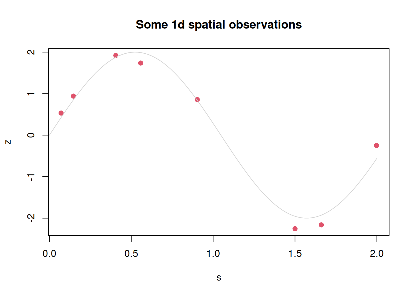
We will illustrate the basic ideas with a simple synthetic 1d example. Note that 1d examples are not unrealistic, since transect sampling is widely used in some spatial applications. Here we will just create a small number of synthetic observations in 1d.
n=8# number of observationss=runif(n, 0, 2)# random observation sitesz=2*sin(3*s)+0.2*rnorm(n)# some fake observationsplot(s, z, pch=19, col=2, main="Some 1d spatial observations")curve(2*sin(3*x), 0, 2, add=TRUE, col="lightgrey")
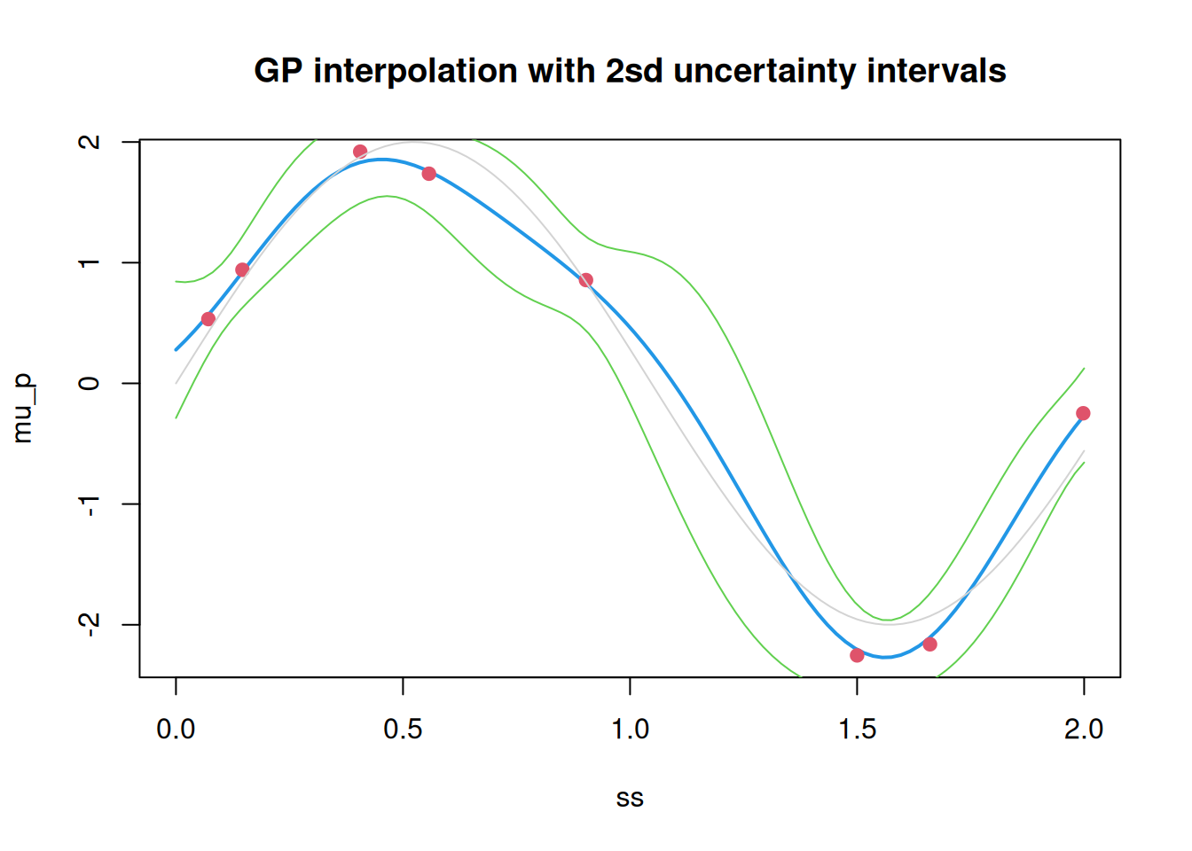
A typical statistical problem is to try to make a prediction for the unobserved latent field using the sparse (and noisy) observations. If we can describe our prior belief about the unobserved field using a fully specified GP, we can use GP regression to solve this problem. Here, we use a mean-zero GP with a squared-exponential covariance, with stationary variance 1 and length scale 0.4. We can set up the joint covariance matrix as follows.
m=100# grid resolution (for unobserved locations of interest)ss=seq(0, 2, length =m)s_all=c(ss, s)# combined vector of unobserved and observed locationsd=as.matrix(dist(s_all))# full joint distance matrixcf=function(h, phi)# squared exponential covarianceexp(-(h/phi)^2)C_all=cf(d, 0.4)# full joint covariance matrixnv=0.2^2# nugget variance (can be 0)C_all[(m+1):(m+n), (m+1):(m+n)]=C_all[(m+1):(m+n), (m+1):(m+n)]+nv*diag(n)
We now use MVN conditioning to compute the posterior distribution given the observations.
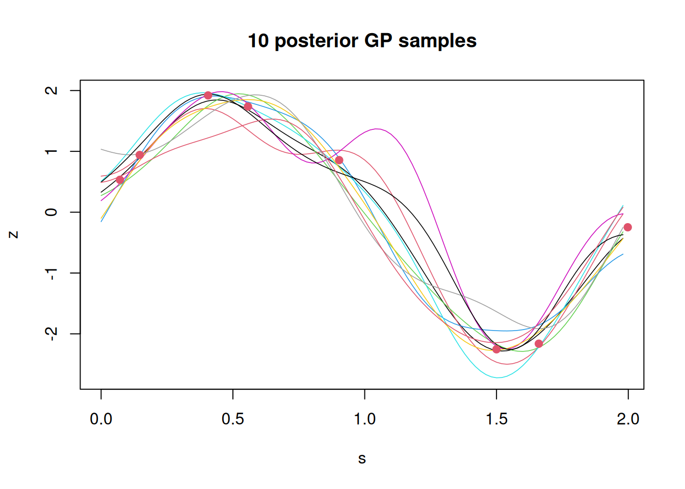
Note that the uncertainty is smallest in the vicinity of the observations. Also note that in this artificial situation where we actually know the true latent field, the uncertainty bands do contain the truth. The mean function is a smoothed prediction of the latent field, but is not a plausible realisation of the latent field. It is sometimes useful to generate realisations from the posterior GP to get an understanding of the range of different “possible worlds” that are consistent with the observations.
The samples can also be useful in the context of certain (parameter) inference algorithms.
11.6.2 Posterior mean and covariance function
Since the GP conditioned on measured observations is another GP, it must be characterised by a mean and covariance function. Although we have explained how to compute the distribution at any finite number of sites, we haven’t written down an explicit mean and covariance function for the posterior GP. For this it will be helpful to define, for any site \(\mathbf{s}\in\mathcal{D}\), the \(n\)-vector \[
\mathbf{c}(\mathbf{s}) = [C(\mathbf{s},\mathbf{s}_1),C(\mathbf{s},\mathbf{s}_2),\ldots,C(\mathbf{s},\mathbf{s}_n)]^\top.
\] Now, by considering the posterior mean of a single unobserved site, \(\mathbf{s}\), we get the posterior mean function \[
\mu_P(\mathbf{s}) = \mu(\mathbf{s}) + \mathbf{c}(\mathbf{s})^\top(\mathsf{\Sigma}_O+\sigma^2\mathbb{I})^{-1}(\mathbf{z}-\pmb{\mu}_O).
\] Similarly, by considering the posterior variance for a pair of sites \(\mathbf{s}\), \(\mathbf{s}'\) and focusing on the off-diagonal element, we get the posterior covariance function \[
C_P(\mathbf{s},\mathbf{s}') = C(\mathbf{s},\mathbf{s}') - \mathbf{c}(\mathbf{s})^\top(\mathsf{\Sigma}_O+\sigma^2\mathbb{I})^{-1} \mathbf{c}(\mathbf{s}').
\] Note that this posterior GP will not be (intrinsically) stationary, even if the prior GP is. It can sometimes be convenient to use the mean and covariance functions directly for prediction and uncertainty quantification in situations where there is interest in making predictions for the latent field at a very large number of sites.
Using GP regression for smoothing and interpolation of a latent field based on finitely many observations is a special case of a more general class of techniques usually referred to as Kriging. We will have much more to say about this in Chapter 13.