Calculus by computer

4.2.1 Other FD formulae

The FD approach considered above is forward differencing. Centred differences are more accurate, but more costly…

…in the well scaled case $\Delta \approx \epsilon ^{1/3}$ is about right.

Higher order derivatives can also be useful. For example

which in the well scaled case will be most accurate for $\Delta \approx \epsilon ^{1/4}$.

4.3.1 Reverse mode AD

If you require many derivatives of a scalar valued function then forward mode AD will have a theoretical computational cost similar to finite differencing, since at least as many operations are required for each derivative as are required for function evaluation. In reality the overheads associated with operator overloading make AD more expensive (alternative strategies also carry overheads). Of course the benefit of AD is higher accuracy, and in many applications the cost is not critical.

An alternative with the potential for big computational savings over finite differencing is reverse mode AD. To understand this it helps to think of the evaluation of a function in terms of a computational graph. Again concentrate on the example function given in Nocedal and Wright (2006):

Any computer evaluating this must break the computation down into a sequence of elementary operations on one or two floating point numbers. This can be thought of as a graph:

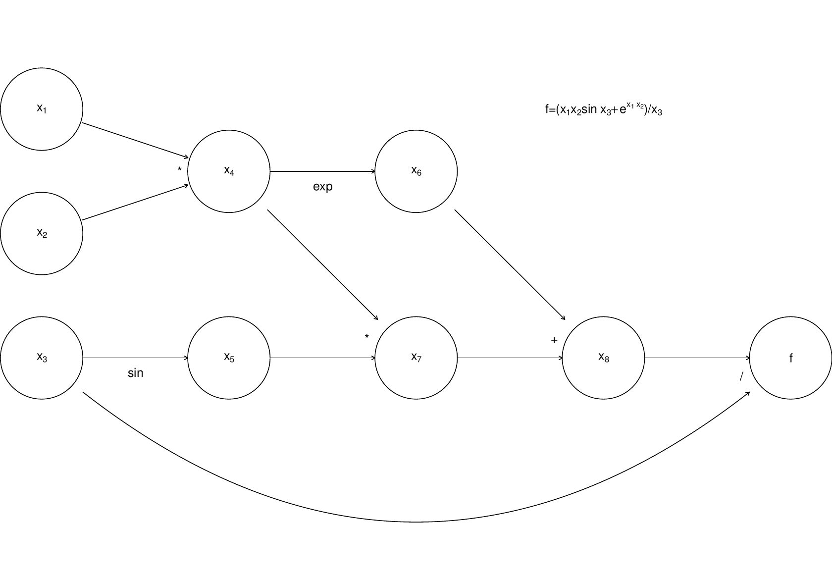
where the nodes $x_4$ to $x_8$ are the intermediate quantities that will have to be produced en route from the input values $x_1$ to $x_3$ to the final answer, $f$. The arrows run from parent nodes to child nodes. No child can be evaluated until all its parents have been evaluated.

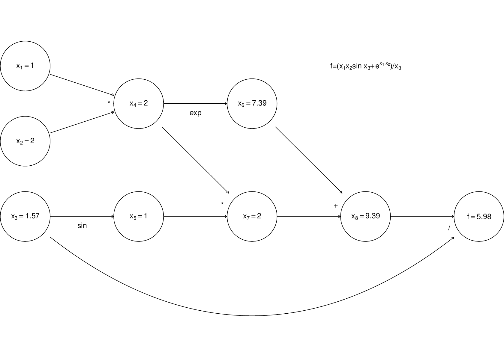
Simple left to right evaluation of this graph results in this …

Now, forward mode AD carries derivatives forward through the graph, alongside values. e.g. the derivative of a node with respect to input variable, $x_1$ is computed using

(the r.h.s. being evaluated by overloaded functions and operators, in the object oriented approach). The following illustrates this process, just for the derivative w.r.t. $x_1$.

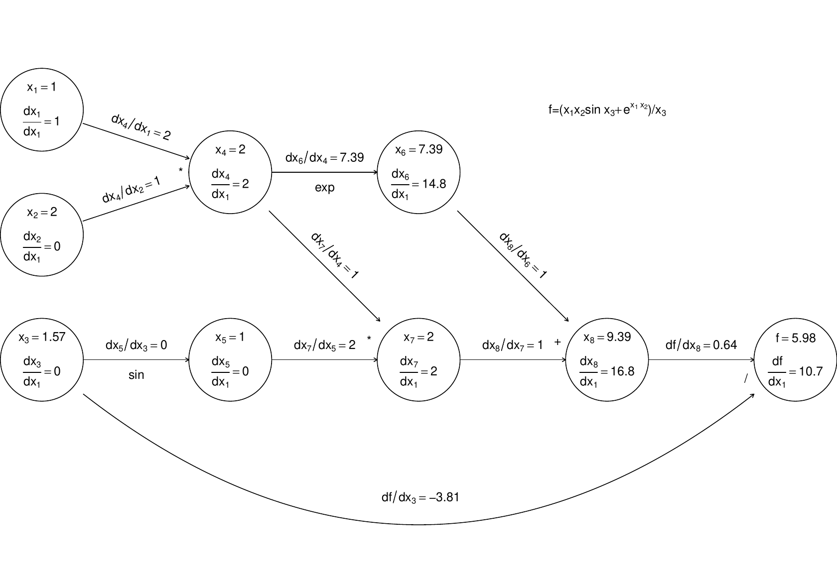
…Again computation runs left to right, with evaluation of a node only possible once all parent values are known.

Now, if we require derivatives w.r.t. several input variables, then each node will have to evaluate derivatives w.r.t. each of these variables, and this becomes expensive (in terms of the previous graph, each node would contain multiple evaluated derivatives). Reverse mode therefore does something ingenious. It first executes a forward sweep through the graph, evaluating the function and all the derivatives of nodes w.r.t. their parents, as follows:

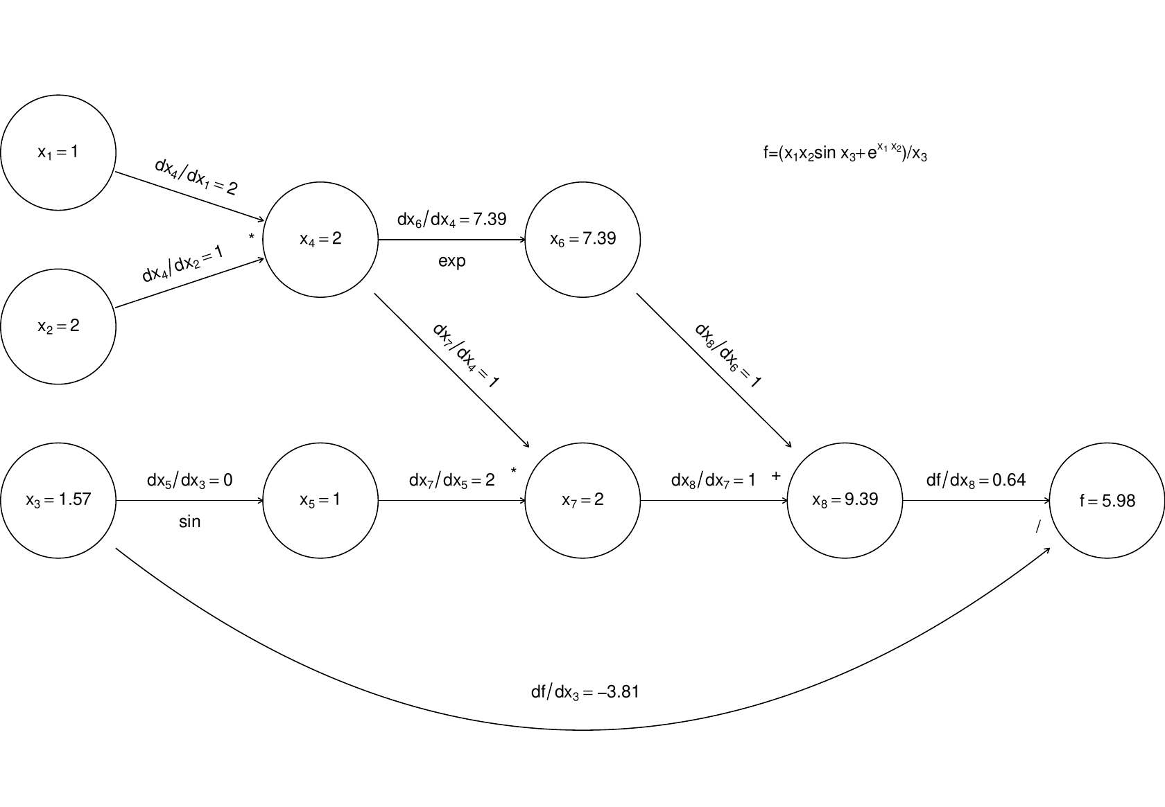
The reverse sweep then works backwards through the graph, evaluating the derivative of $f$ w.r.t. each node, using the following

and the fact that at the terminal node $\partial f/{\partial f } = 1$.

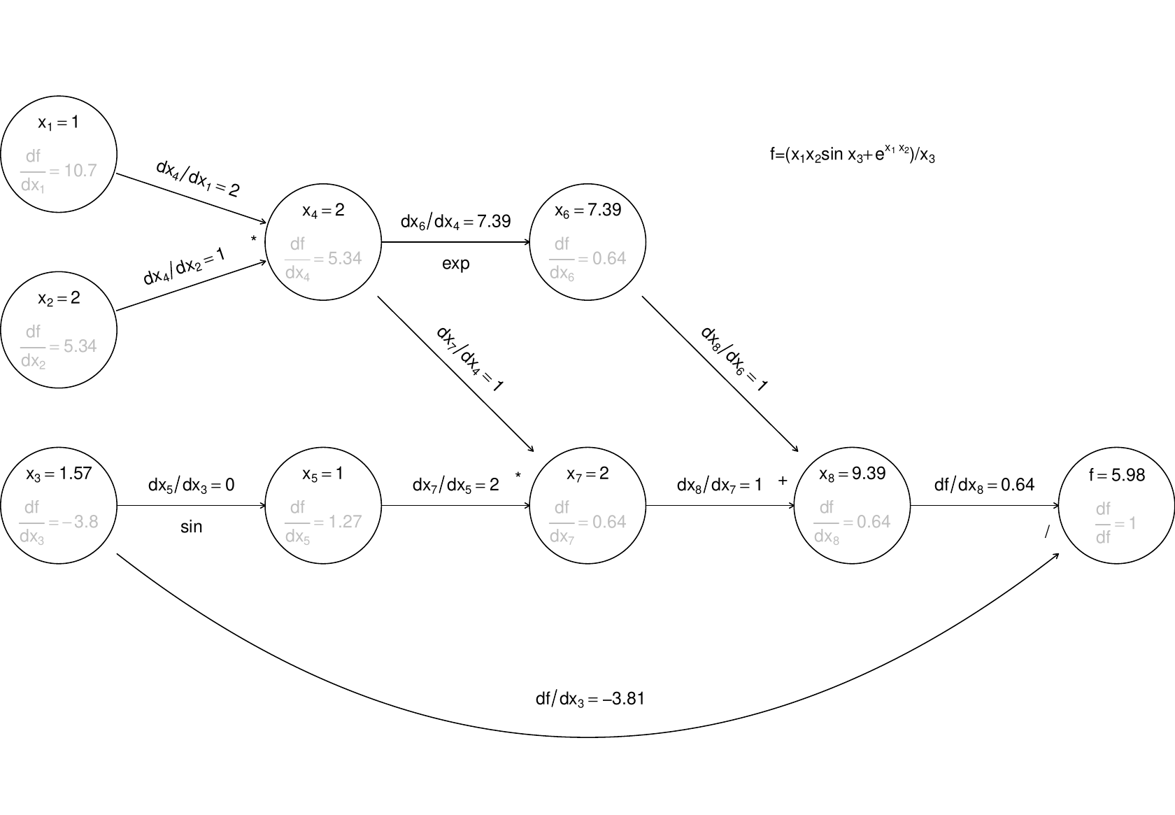
The derivatives in grey are those calculated on the reverse sweep. The point here is that there is only one derivative to be evaluated at each node, but in the end we know the derivative of $f$ w.r.t. every input variable. Reverse mode can therefore save a large number of operations relative to finite differencing or forward mode. Once again, general purpose AD libraries automate the process for you, so that all you need to be able to write is the evaluation code.

Unfortunately reverse mode efficiency comes at a heavy price. In forward mode we could discard the values and derivatives associated with a node as soon as all its children were evaluated. In reverse mode the values of all nodes and the evaluated derivatives associated with every connection have to be stored during the forward sweep, in order to be used in the reverse sweep. This is a heavy storage requirement. For example, if $f$ involved the inversion of a $1000\times 1000$ matrix then we would have to store some $2 \times 10^9$ intermediate node values plus a similar number of evaluated derivatives. That is some 32 Gigabytes of storage before we even consider the requirements for storing the structure of the graph.

4.3.2 A caveat

For AD to work it is not sufficient that the function being evaluated has properly defined derivatives at the evaluated function value. We require that every function/operator used in the evaluation has properly defined derivatives at its evaluated argument(s). This can create a problem with code that executes conditional on the value of some variable. For example the Box-Cox transformation of a positive datum $y$ is

If you code this up in the obvious way then AD will never get the derivative of $B$ w.r.t. $\lambda$ right if $\lambda = 0$.

4.3.3 Using AD to improve FD

When fitting complicated or computer intensive models it can be that AD is too expensive to use for routine derivative calculation during optimisation. However, with the gradual emergence of highly optimised libraries, this situation is changing, and in any case it can still provide a useful means for calibrating FD intervals. A ‘typical’ model run can be auto-differentiated, and the finite difference intervals adjusted to achieve the closest match to the AD derivatives. As optimisation progresses one or two further calibrations of the FD intervals can be carried out as necessary.

4.4.1 Quadrature rules

In one dimension we might choose to approximate the integral of a continuous function $f(x)$ by the area under a set of step functions, with the midpoint of each matching $f$:

where $h$ in the final error term is $(b-a)/N$. Let’s see what the error bound means in practice by approximating $\int _0^1 e^ x dx$.

  I.true <- exp(1) - 1
  N <- 10
  I.mp <- sum(exp((1:N-.5)/N))/N
  c(I.mp,I.true,(I.true-I.mp)/I.true)

## [1] 1.7175660865 1.7182818285 0.0004165452

  N <- 100
  I.mp <- sum(exp((1:N-.5)/N))/N
  c(I.mp,I.true,(I.true-I.mp)/I.true)

## [1] 1.718275e+00 1.718282e+00 4.166655e-06

  N <- 1000
  I.mp <- sum(exp((1:N-.5)/N))/N
  c(I.mp,I.true,(I.true-I.mp)/I.true)

## [1] 1.718282e+00 1.718282e+00 4.166667e-08

If $f$ is cheap to evaluate, accuracy is not paramount and we are only interested in 1 dimensional integrals then we might stop there (or more likely with the slightly more accurate but equally straightforward ‘Simpson’s Rule’), but life is not so simple. If one is very careful about the choice of $x$ points at which to evaluate $f(x)$ and about the weights used in the integral approximating summation, then some very impressive results can be obtained, at least for smooth enough functions, using Gauss(ian) Quadrature. The basic idea is to find a set $\{ x_ i, w_ i:i=1,\ldots ,n\}$ such that if $w(x)$ is a fixed weight function and $g(x)$ is any polynomial up to order $2n-1$ then

Note that the $x_ i, w_ i$ set depends on $w(x)$, $a$ and $b$, but not on $g(x)$. The hope is that the r.h.s. will still approximate the l.h.s. very accurately if $g(x)$ is not a polynomial of the specified type, and there is some impressive error analysis to back this up, for any function with $2n$ well behaved derivatives (see e.g. Monahan, 2001, section 10.3).

The R package statmod has a nice gauss.quad function for producing the weights, $w_ i$ and nodes, $x_ i$, for some standard $w(x)$s. It assumes $a=-1$, $b=1$, but we can just linearly re-scale our actual interval to use this. Here is the previous example using Gauss Quadrature (assuming $w(x)$ is a constant).

library(statmod)
N <- 10
gq <- gauss.quad(N) # get the x_i, w_i
gq # take a look

## $nodes
##  [1] -0.9739065 -0.8650634 -0.6794096 -0.4333954 -0.1488743  0.1488743
##  [7]  0.4333954  0.6794096  0.8650634  0.9739065
## 
## $weights
##  [1] 0.06667134 0.14945135 0.21908636 0.26926672 0.29552422 0.29552422
##  [7] 0.26926672 0.21908636 0.14945135 0.06667134

sum(gq$weights) # for an interval of width 2

## [1] 2

I.gq <- sum(gq$weights*exp((gq$nodes+1)/2))/2
c(I.gq, I.true, (I.true-I.gq)/I.true)

## [1]  1.718282e+00  1.718282e+00 -1.292248e-15

gqi <- function(g, N = 10, a = -1, b = 1) {
    gq = gauss.quad(N)
    w = gq$weights*(b-a)/2
    n = a + (b-a)*(gq$nodes + 1)/2
    sum(w * g(n))
    }

gqi(exp, 10, 0, 1)

## [1] 1.718282

I.gq <- gqi(exp, 5, 0, 1)
c(I.gq, I.true, (I.true-I.gq)/I.true)

## [1] 1.718282e+00 1.718282e+00 3.805670e-13

I.gq <- gqi(exp, 3, 0, 1)
c(I.gq, I.true, (I.true-I.gq)/I.true)

## [1] 1.718281e+00 1.718282e+00 4.795992e-07

4.4.2 Quadrature rules for multidimensional integrals

We can integrate w.r.t. several variables by recursive application of quadrature rules. For example consider integrating $f(x,z)$ over a square region, and assume we use basically the same node and weight sequence for both dimensions. We have

and so

Clearly, in principle we can repeat this for as many dimensions as we like. In practice however, to maintain a given level of accuracy, the number of function evaluations will have to rise as $N^ d$ where $N$ is the number of nodes for each dimension, and $d$ is the number of dimensions. Even if we can get away with a 3 point Gaussian quadrature, we will need 1.5 million evaluations by the time we reach a 13 dimensional integral.

Here is a function which takes the node sequence x and weight sequence w of some quadrature rule and uses them to produce the d dimensional set of nodes, and the corresponding weight vector resulting from recursive application of the 1D rule.

mesh <- function(x,d,w=1/length(x)+x*0) {
  n <- length(x)
  W <- X <- matrix(0,n^d,d)
  for (i in 1:d) {
   X[,i] <- x;W[,i] <- w
   x <- rep(x,rep(n,length(x)))
   w <- rep(w,rep(n,length(w)))
  }
 w <- exp(rowSums(log(W))) ## column product of W gives weights
 list(X=X,w=w) ## each row of X gives co-ordinates of a node
}

mesh(c(1,2),3)

## $X
##      [,1] [,2] [,3]
## [1,]    1    1    1
## [2,]    2    1    1
## [3,]    1    2    1
## [4,]    2    2    1
## [5,]    1    1    2
## [6,]    2    1    2
## [7,]    1    2    2
## [8,]    2    2    2
## 
## $w
## [1] 0.125 0.125 0.125 0.125 0.125 0.125 0.125 0.125

fd <- function(x) {exp(rowSums(x))}

  N <- 10; d <- 2; N^d # number of function evaluations

## [1] 100

  I.true <- (exp(1)-exp(-1))^d
  mmp <- mesh((1:N-.5)/N*2-1,d,rep(2/N,N))
  I.mp <- sum(mmp$w*fd(mmp$X))
  c(I.mp,I.true,(I.true-I.mp)/I.true)

## [1] 5.506013515 5.524391382 0.003326677

  N <- 10; d <- 5; N^d # number of function evaluations

## [1] 1e+05

  I.true <- (exp(1)-exp(-1))^d
  mmp <- mesh((1:N-.5)/N*2-1,d,rep(2/N,N))
  I.mp <- sum(mmp$w*fd(mmp$X))
  c(I.mp,I.true,(I.true-I.mp)/I.true)

## [1] 71.136612879 71.731695754  0.008295954

Of course Gauss Quadrature is a better bet

  N <- 4; d <- 2; N^d

## [1] 16

  I.true <- (exp(1)-exp(-1))^d
  gq <- gauss.quad(N)
  mgq <- mesh(gq$nodes,d,gq$weights)
  I.gq <- sum(mgq$w*fd(mgq$X))
  c(I.gq,I.true,(I.true-I.gq)/I.true)

## [1] 5.524390e+00 5.524391e+00 2.511325e-07

  N <- 4; d <- 5; N^d

## [1] 1024

  I.true <- (exp(1)-exp(-1))^d
  gq <- gauss.quad(N)
  mgq <- mesh(gq$nodes,d,gq$weights)
  I.gq <- sum(mgq$w*fd(mgq$X))
  c(I.gq,I.true,(I.true-I.gq)/I.true)

## [1] 7.173165e+01 7.173170e+01 6.278311e-07

4.4.3 Approximating the integrand

Beyond a few dimensions, quadrature rules really run out of steam. In statistical work, where we are often interested in integrating probability density functions, or related quantities, it is sometimes possible to approximate the integrand by a function with a known integral. Here, just one approach will be illustrated: Laplace approximation. The typical application of the method is when we have a joint density $f({\bf y},{\bf b})$ and want to evaluate the marginal p.d.f. of $\bf y$,

For a given $\bf y$ let $\hat{\bf b}_ y$ be the value of $\bf b$ maximising $f$. Then Taylor’s theorem implies that

where $\bf H$ is the Hessian of $-\log (f)$ w.r.t. $\bf b$ evaluated at ${\bf y}, \hat{\bf b}_ y$. i.e.

and so

From the properties of normal p.d.f.s we have

so

Notice that the basic ingredients of this approximation are the Hessian of the log integrand w.r.t ${\bf b}$ and the $\hat{\bf b}_ y$ values. Calculating the latter is an optimisation problem, which can usually be solved by a Newton type method, given that we can presumably obtain gradients as well as the Hessian. The highest cost here is the Hessian calculation, which scales with the square of the dimension, at worst, or for cheap integrands the determinant evaluation, which scales as the cube of the dimension. i.e. when it works, this approach is much cheaper than brute force quadrature.

4.4.4 Monte-Carlo integration

Consider integrating $f({\bf x})$ over some region $\Omega$ of volume $V(\Omega )$. Clearly

where ${\bf X} \sim$ uniform over $\Omega$. Generating $N$ uniform random vectors, ${\bf x}_ i$, over $\Omega$, we have the obvious estimator

which defines basic Monte-Carlo Integration. ³ Clearly $\hat I_\Omega$ is unbiased, and if the ${\bf x}_ i$ are independent then

i.e. the variance scales as $N^{-1}$, and the standard deviation scales as $N^{-1/2}$ (it’s $O_ p(N^{-1/2})$). This is not brilliantly fast convergence to $I_\Omega$, but compare it to quadrature. If we take the midpoint rule then the (bias) error is $O(h^2)$ where $h$ is the node spacing. In $d$ dimensions then at best we can arrange $h \propto N^{-1/d}$, implying that the bias is $O(N^{-2/d})$. i.e. once we get above $d=4$ we would prefer the stochastic convergence rate of Monte-Carlo Integration to the deterministic convergence rate of the midpoint rule.

Of course using Simpson’s rule would buy us a few more dimensions, and for smooth functions the spectacular convergence rates of Gauss quadrature may keep it as the best option up to a rather higher $d$, but the fact remains that its bias is still dependent on $d$, while the sampling error of the Monte Carlo method is dimension independent, so Monte Carlo will win in the end.

4.4.5 Stratified Monte-Carlo Integration

One tweak on basic Monte-Carlo is to divide (a region containing) $\Omega$ into $N$ equal volumed sub-regions, $\Omega _ i$, and to estimate the integral within each $\Omega _ i$ from a single ${\bf X}_ i$ drawn from a uniform distribution over $\Omega _ i$. The estimator has the same form as before, but its variance is now

which is usually lower than previously, because the range of variation of $f$ within each $\Omega _ i$ is lower than within the whole of $\Omega$.

The underlying idea of trying to obtain the nice properties of uniform random variables, but with more even spacing over the domain of integration, is pushed to the limit by Quasi-Monte-Carlo integration, which uses deterministic space filling sequences of numbers as the basis for integration. For fixed $N$, the bias of such schemes grows much less quickly with dimension than the quadrature rules.

4.4.6 Importance sampling

In statistics an obvious variant on Monte-Carlo integration occurs when the integrand factors into the product of a p.d.f. $f({\bf x})$ and another term in which case

where the ${\bf x}_ i$ are observations on r.v.s with p.d.f. $f({\bf x})$. A difficulty with this approach, as with simple MC integration, is that a high proportion of the ${\bf x}_ i$s often fall in places where $\phi ({\bf x}_ i)$ makes no, or negligible, contribution to the integral. For example, in Bayesian modelling, it is quite possible for the $f({\bf y}|{\bm \theta })$ to be have non-vanishing support over only a tiny volume of the parameter space over which $f({\bm \theta })$ has non-vanishing support.

One approach to this problem is importance sampling. Rather than generate the ${\bf x}_ i$ from $f({\bf x})$ we generate from a distribution with the same support as $f$, but with a p.d.f., $g({\bf x})$, which is designed to generate points concentrated in the places where the integrand is non-negligible. Then the estimator is

The expected value of the r.h.s. of the above is its l.h.s., so this estimator is unbiased.

What would make a good $g$? Suppose that $g \propto \phi f$. Then $g({\bf x}) = \phi ({\bf x}) f({\bf x})/k$, where $k = \int \phi ({\bf x}) f({\bf x}) d{\bf x}$. So $\hat I_{is} = nk/n = \int \phi ({\bf x}) f({\bf x}) d{\bf x}$, and the estimator has zero variance. Clearly this is impractical. If we knew $k$ then we would not need to estimate, but there are useful insights here anyway. Firstly, the more constant is $\phi f/g$, the lower the variance of $\hat I_{is}$. Secondly, the idea that the density of evaluation points should reflect the contribution of the integrand in the local neighbourhood is quite generally applicable.

4.4.7 Laplace importance sampling

We are left with the question of how to choose $g$? When the integrand is some sort of probability density function, a reasonable approach is to approximate it by the normal density implied by the Laplace approximation. That is we take $g$ to be the p.d.f. of the multivariate normal $N(\hat{\bf x},{\bf H}^{-1})$ where $\hat{\bf x}$ denotes the ${\bf x}$ value maximising $\phi f$, while $\bf H$ is the Hessian of $-\log (\phi f)$ w.r.t. $\bf x$, evaluated at $\hat{\bf x}$.

In fact, as we have seen previously, multivariate normal random vectors are generated by transformation of standard normal random vectors ${\bf z} \sim N({\bf 0},{\bf I})$. i.e. ${\bf x} = \hat{\bf x} + {\bf R}^{-1}{\bf z}$ where ${\bf R}$ is a Cholesky factor of $\bf H$ so that ${\bf R}^{\sf T}{\bf R} = {\bf H}$. There is then some computational saving in using a change of variable argument to re-express the importance sampling estimator in terms of the density of $\bf z$, rather than $g$ itself. Start with

where $h({\bf z}) = (2\pi )^{-d/2}\exp \{ -{\bf z}^{\sf T}{\bf z}/2\}$ is the standard normal density for ${\bf z}$, giving

and leading in turn to the Laplace importance sampling estimator

Some tweaks may be required.

1. 1.

   It might be desirable to make $g$ a little more diffuse than the Laplace approximation suggests, to avoid excessive importance weights being assigned to ${\bf z}_ i$ values in the tails of the target distribution.

2. 2.

   If the integration is in order to obtain a likelihood, which is to be maximised, then it is usually best to condition on a set of ${\bf z}_ i$ values, in order to avoid random variability in the approximate likelihood, which will make optimisation difficult.

3. 3.

   Usually the log of the integrand is evaluated rather than the integrand itself, and it is the log of the integral that is required. To avoid numerical under/overflow problems note that

   $$\log \left\{ \sum _ i w_ i \exp (\psi _ i) \right\} = \log \left[\sum _ i w_ i \exp \{ \psi _ i - \max (\psi _ i)\} \right] + \max (\psi _ i)$$

   the r.h.s. will not overflow or underflow when computed in finite precision arithmetic (for reasonable $w_ i$).

4. 4.

   As with simple Monte-Carlo integration, some variance reduction is achievable by stratification. The ${\bf z}_ i$ can be obtained by suitable transformation of random vectors from a uniform distribution on $(0,1)^ d$. Instead $(0,1)^ d$ can be partitioned into equal volume parts, with one uniform vector generated in each…

Tweak 3. is an example of a general technique for avoiding numerical underflow and overflow which has many applications in statistical computing. It is therefore worth examining more carefully.

4.4.8 The log–sum–exp trick

In statistical computing, we rarely want to work with raw probabilities and likelihoods, but instead work with their logarithms. Log-likelihoods are much less likely to numerically underflow or overflow than raw likelihoods. For likelihood computations involving iid observations, this is often convenient, since a product of raw likelihood terms becomes a sum of log-likelihood terms. However, sometimes we have to evaluate the sum of raw probabilities or likelihoods. The obvious way to do this would be to exponentiate the logarithms, evaluate the sum, and then take the log of the result to get back to our log scale. However, the whole point to working on the log scale is to avoid numerical underflow and overflow, so we know that exponentiating raw likelihoods is a dangerous operation which is likely to fail in many problems. Can we do the log–sum–exp operation safely? Yes, we can.

Suppose that we have log (unnormalised) weights (typically probabilities or likelihoods), $l_ i = \log w_ i$, but we want to compute the (log of the) sum of the raw weights. We can obviously exponentiate the log weights and sum them, but this carries the risk that all of the log weights will underflow (or, possibly, overflow). So, we want to compute

without the risk of underflow. We can do this by first computing $m = \max _ i l_ i$ and then noting that

We are now safe, since $l_ i-m$ cannot be bigger than zero, and hence no term can overflow. Also, since we know that $l_ i-m = 0$ for some $i$, we know that at least one term will not underflow to zero. So we are guaranteed to get a sensible finite answer in a numerically stable way. Note that exactly the same technique works for computing a sample mean (or other weighted sum) as opposed to just a simple sum (as above).

4.4.9 An example

Consider a Generalised Linear Mixed Model:

where $\bm \Lambda$ is diagonal and depends on a small number of parameters. Here, ${\bm \beta }$ are the fixed effects and ${\bf b}$ are the random effects, with covariate matrices ${\bf X}$ and ${\bf Z}$, respectively. From the model specification it is straightforward to write down the joint probability function of $\bf y$ and $\bf b$, based on the factorisation $f({\bf y}, {\bf b}) = f_{y|b}({\bf y}|{\bf b})f_ b({\bf b})$. i.e.

but likelihood based inference actually requires that we can evaluate the marginal p.f. $f_ y({\bf y})$ for any values of the model parameters. Now

and evaluation of this requires numerical integration.

To tie things down further, suppose that the fixed effects part of the model is simply $\beta _0 + \beta _1 x$ where $x$ is a continuous covariate, while the random effects part is given by two factor variables, $z_1$ and $z_2$, each with two levels. So a typical row of ${\bf Z}$ is a vector of 4 zeros and ones, in some order. Suppose further that the first two elements of $\bf b$ relate to $z_1$ and the remainder to $z_2$ and that ${\rm diag}({\bm \Lambda }) = [\sigma ^{-2}_1,\sigma ^{-2}_1,\sigma ^{-2}_2,\sigma ^{-2}_2]$. The following simulates 50 observations from such a model.

set.seed(0);n <- 50
x <- runif(n)
z1 <- sample(c(0,1),n,replace=TRUE)
z2 <- sample(c(0,1),n,replace=TRUE)
b <- rnorm(4) ## simulated random effects
X <- model.matrix(~x)
Z <- cbind(z1,1-z1,z2,1-z2)
eta <- X%*%c(0,3) + Z%*%b
mu <- exp(eta)
y <- rpois(n, mu)

lf.yb0 <- function(y, b, theta, X, Z, lambda) {
  beta <- theta[1:ncol(X)]
  theta <- theta[-(1:ncol(X))]
  eta <- X%*%beta + Z%*%b
  mu <- exp(eta)
  lam <- lambda(theta, ncol(Z))
  sum(y*eta - mu - lfactorial(y)) - sum(lam*b^2)/2 +
      sum(log(lam))/2 - ncol(Z)*log(2*pi)/2
}

theta contains the fixed effect parameters, i.e. ${\bm \beta }$ and the parameters of $\bm \Lambda$. So in this example, theta is of length 4, with the first 2 elements corresponding to ${\bm \beta }$ and the last two are $\sigma _1^{-2}, \sigma _{2}^{-2}$. lambda is the name of a function for turning the parameters of $\bm \Lambda$ into its leading diagonal elements, for example

var.func <- function(theta, nb) c(theta[1], theta[1],
                                    theta[2], theta[2])

  theta <- c(0,3,1,1)
  nm <- 10;m.r <- 10
  bm <- mesh((1:nm-(nm+1)/2)*m.r/nm,4,rep(m.r/nm,nm))
  lf <- lf.yb(y,t(bm$X),theta,X,Z,var.func)
  log(sum(bm$w*exp(lf-max(lf)))) + max(lf)

## [1] -116.5303

  log(sum(bm$w*exp(lf-max(lf)))) + max(lf)

## [1] -118.6234

  nm <- 10
  gq <- gauss.quad(nm)
  w <- gq$weights*m.r/2 ## rescale to domain
  x <- gq$nodes*m.r/2
  bm <- mesh(x,4,w)
  lf <- lf.yb(y,t(bm$X),theta,X,Z,var.func)
  log(sum(bm$w*exp(lf-max(lf)))) + max(lf)

## [1] -136.95

  log(sum(bm$w*exp(lf-max(lf)))) + max(lf)

## [1] -125.3369

b <- rep(0,4)
while(TRUE) {
  b0 <- b
  g <- glf.yb(y, b, theta, X, Z, var.func)
  H <- hlf.yb(y, b, theta, X, Z, var.func)
  b <- b - solve(H, g)
  b <- as.vector(b)
  if (sum(abs(b-b0)) < 1e-5*sum(abs(b)) + 1e-4) break
}

lf.yb0(y,b,theta,X,Z,var.func) + 2*log(2*pi) -
    0.5*determinant(H,logarithm=TRUE)$modulus

## [1] -116.9646
## attr(,"logarithm")
## [1] TRUE

  N <- 100000
  bm <- matrix((runif(N*4)-.5)*m.r,4,N)
  lf <- lf.yb(y, bm, theta, X, Z, var.func)
  log(sum(exp(lf-max(lf)))) + max(lf) - log(N) + log(m.r^4)

## [1] -119.8479

## [1] -119.3469

lf.ygb <- function(y, b, theta, X, Z, lambda) {
  beta = theta[1:ncol(X)]
  eta = Z%*%b + as.vector(X%*%beta)
  colSums(y*eta - exp(eta) - lfactorial(y))
}
N = 100000
lam = var.func(theta[3:4])
bm = matrix(rnorm(4*N, 0, sqrt(lam)), nrow=4)
llv = lf.ygb(y, bm, theta, X, Z, var.func)
max(llv) + log(mean(exp(llv - max(llv))))

## [1] -119.2791

## [1] -119.0786

N <- 10000
  R <- chol(-H)
  z <- matrix(rnorm(N*4),4,N)
  bm <- b + backsolve(R,z)
  lf <- lf.yb(y,bm,theta,X,Z,var.func)
  zz.2 <- colSums(z*z)/2
  lfz <- lf + zz.2
  log(sum(exp(lfz - max(lfz)))) + max(lfz) + 2 * log(2*pi) -
      sum(log(diag(R))) - log(N)

## [1] -119.3229

## [1] -119.2882
## [1] -119.2774