Optimisation
Many problems in statistics can be characterised as solving
where is a real scalar valued function of vector , usually known as the objective function. For example: might be the negative log-likelihood of the parameters of a statistical model, the maximum likelihood estimates of which are required; in a Bayesian setting might be a (negative) posterior distribution for , the posterior modes of which are required; might be a dissimilarity measure for the alignment of two DNA sequences, where the alignment is characterised by a parameter vector ; might be total distance travelled, and a vector giving the order in which a delivery van should visit a set of drop off points. Note that maximising is equivalent to minimising so we are not losing anything by concentrating on minimisation here. In the optimisation literature, the convention is to minimise an objective, with the idea being that the objective is some kind of cost or penalty to be minimised. Indeed, the objective function is sometimes referred to as the cost function.
Let denote the set of all possible values. Before discussing specific methods, note that in practice we will only be able to solve (3.1) if one of two properties holds.
-
1.
It is practical to evaluate for all elements of .
-
2.
It is possible to put some structure onto , giving a notion of distance between any two elements of , such that closeness in implies closeness in value.
In complex situations, requiring complicated stochastic approaches, it is easy to lose sight of point 2 (although if it isn’t met we may still be able to find ways of locating values that reduce ).
Optimisation problems vary enormously in difficulty. In the matrix section we saw algorithms with operation counts which might be proportional to as much as . There are optimisation problems whose operations count is larger than for any : in computer science terms there is no polynomial time algorithm 1 for solving them. Most of these really difficult problems are discrete optimisation problems, in that takes only discrete values, rather than consisting of unconstrained real numbers. One such problem is the famous Travelling salesman problem, which concerns finding the shortest route between a set of fixed points, each to be visited only once. Note however, that simply having a way of improving approximate solutions to such problems is usually of considerable practical use, even if exact solution is very taxing.
Continuous optimisation problems in which is a real random vector are generally more straightforward than discrete problems, and we will concentrate on such problems here. In part this is because of the centrality of optimisation methods in practical likelihood maximisation.
3.1 Local versus global optimisation
Minimisation methods generally operate by seeking a local minimum of . That is they seek a point, , such that , for any sufficiently small perturbation . Unless is a strictly convex function, it is not possible to guarantee that such a is a global minimum. That is, it is not possible to guarantee that for any arbitrary .
3.2 Optimisation methods are myopic
Before going further it is worth stressing another feature of optimisation methods: they are generally very short-sighted. At any stage of operation all that optimisation methods ‘know’ about a function are a few properties of the function at the current best , (and, much less usefully, those same properties at previous best points). It is on the basis of such information that a method tries to find an improved best . The methods have no ‘overview’ of the function being optimised.
3.3 Look at your objective first
Before attempting to optimise a function with respect to some parameters, it is a good idea to produce plots in order to get a feel for the function’s behaviour. Of course if you could simply plot the function over the whole of it is unlikely that you would need to worry about numerical optimisation, but generally this is not possible, and the best that can be achieved is to look at some one or two dimensional transects through .
To fix ideas, consider the apparently innocuous example of fitting a simple dynamic model to a single time series by least squares/maximum likelihood. The dynamic model is
where and are parameters and we will assume that is known. Further suppose that we have observations where . Estimation of and by least squares (or maximum likelihood, in this case) requires minimisation of
w.r.t. and . We should try to get a feel for the behaviour of . To see how this can work consider some simulated data examples. In each case I used , and for the simulations, but I have varied between the cases.
-
In the first instance data were simulated with . If we now pretend that we need to estimate and from such data, then we might look at some -transects and some -transects through . This figure shows the raw data and an -transect.
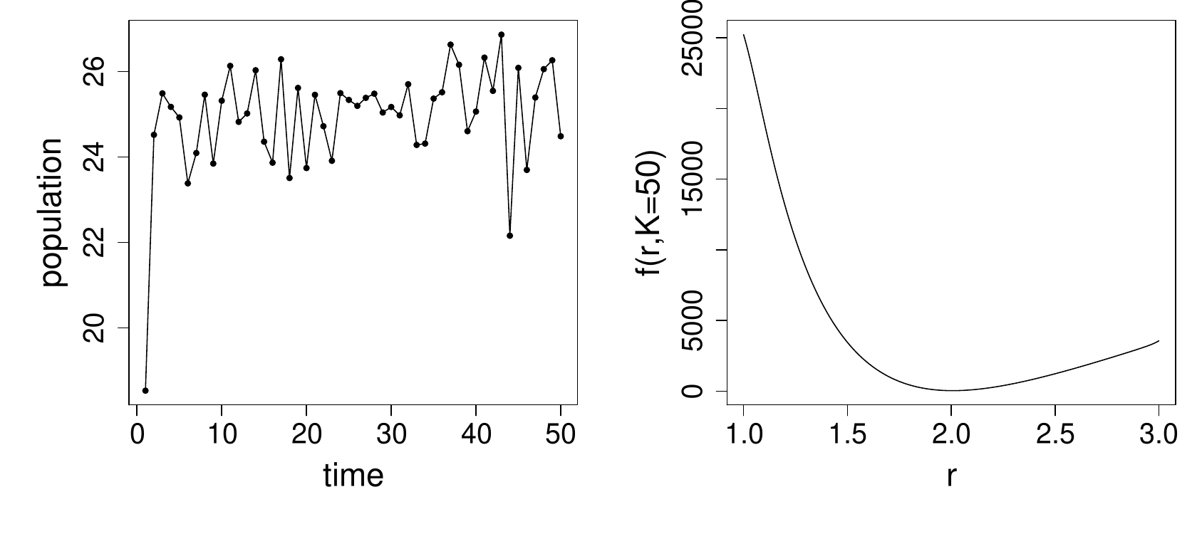
-transects with other values look equally innocuous, and -transects also look benign over this range. So in this case appears to be a nice smooth function of and , and any half decent optimisation method ought to be able to find the optimum.
-
In the second example data were simulated with . Again pretend that we only have the data and need to estimate and from it. Examination of the left hand plot below, together with some knowledge of the model’s dynamic behaviour, indicates that is probably in the 3 to 4 range.
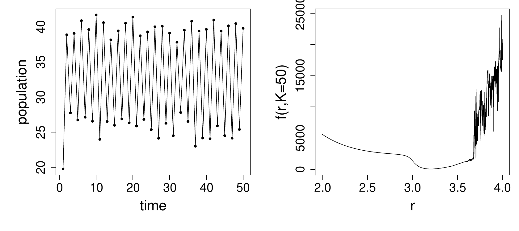
Notice that still seems to behave smoothly in the vicinity of its minimum, which is around 3.2, but that something bizarre starts to happen above 3.6. Apparently we could be reasonably confident of locating the function’s minimum if we start out below or reasonably close to 3.2, but if we stray into the territory above 3.6 then there are so many local minima that locating the desired global minimum would be very difficult.
-
Finally data were simulated with .
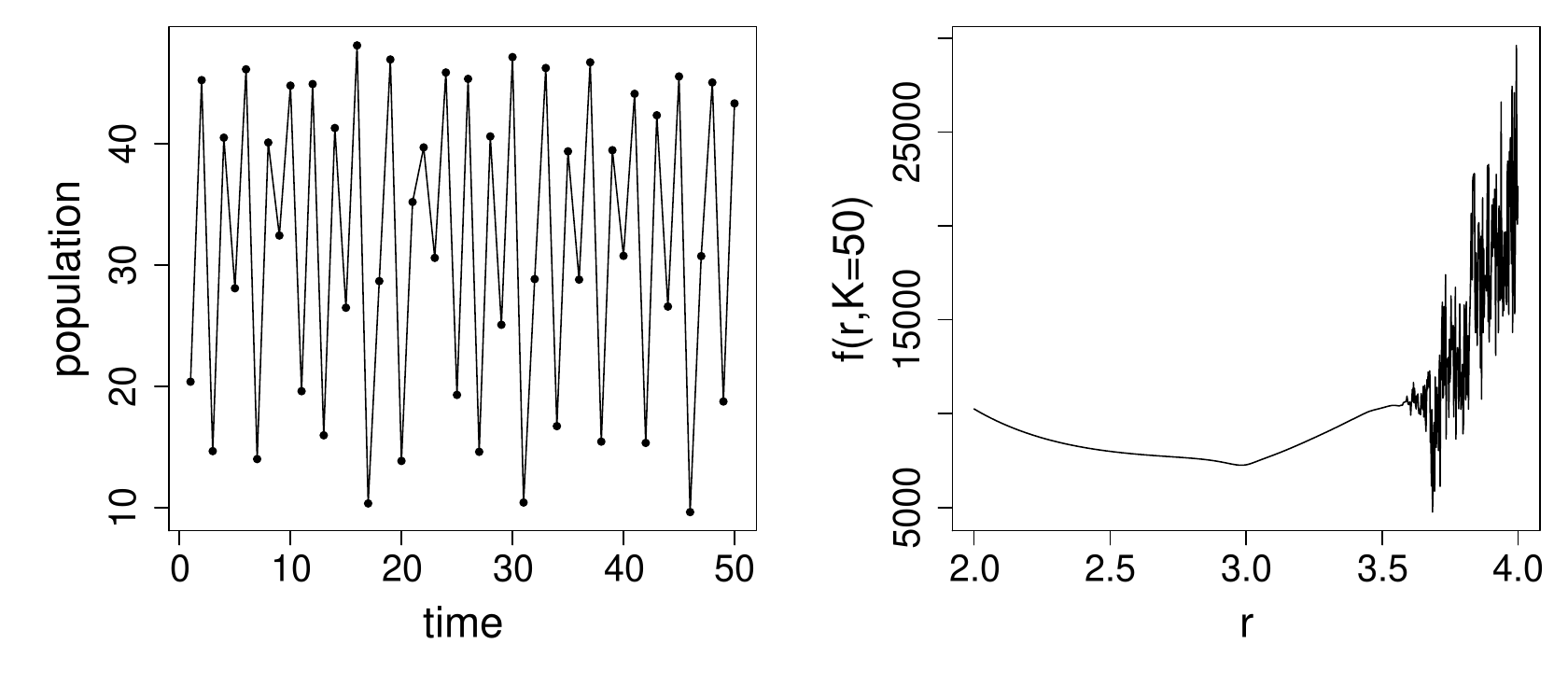
Now the objective has a minimum somewhere around 3.7, but it is surrounded by other local minima, so that locating the actual minima would be a rather taxing problem. In addition it is now unclear how we would go about quantifying uncertainty about the ‘optimal’ : it will certainly be of no use appealing to asymptotic likelihood arguments in this case.
So, in each of these examples, simple transects through the objective function have provided useful information. In the first case everything seemed OK. In the second we would need to be careful with the optimisation, and careful to examine how sensible the optimum appeared to be. In the third case we would need to think very carefully about the purpose of the optimisation, and about whether a re-formulation of the basic problem might be needed.
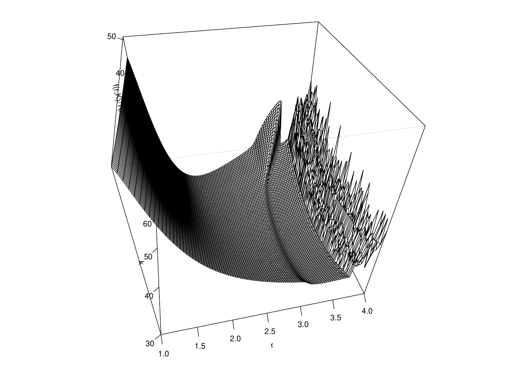
Notice how the behaviour of the objective was highly parameter dependent here, something that emphasises the need to understand models quite well before trying to fit them. In this case the dynamic model, although very simple, can show a wide range of complicated behaviour, including chaos. In fact, for this simple example, it is possible to produce a plot of the fitting objective over pretty much the whole plausible parameter space. Here is an example when data were simulated with
3.3.1 Objective function transects are a partial view
Clearly plotting some transects through your objective function is a good idea, but they can only give a limited and partial view when the is multidimensional. Consider this -transect through a function,
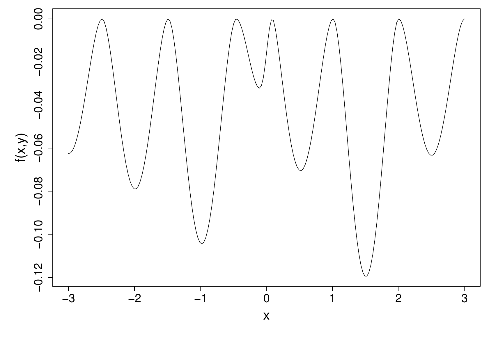
Apparently the function has many local minima, and optimisation will be difficult. Actually the function is this…
It has one local minimum, its global minimum. Head downhill from any point and you will eventually reach the minimum.
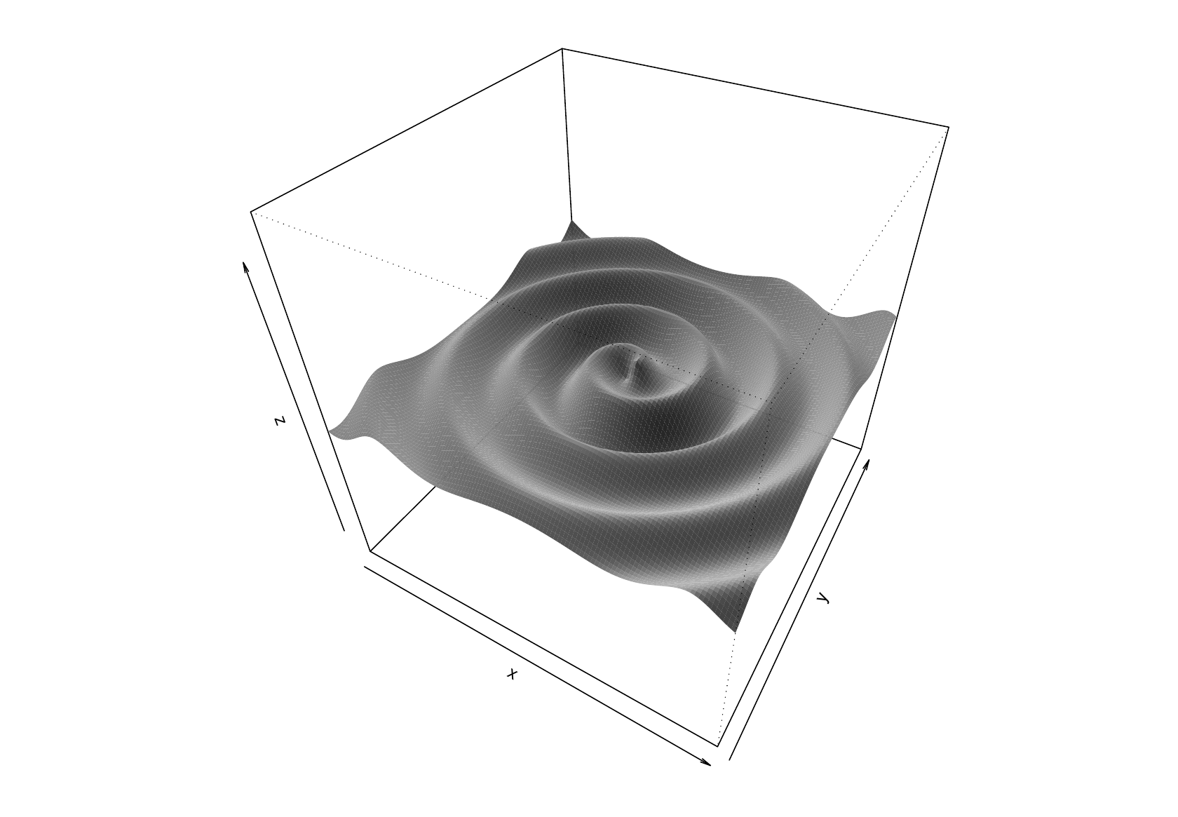
The opposite problem can also occur. Here are and transects through a second function .
…apparently no problem. From these plots you would be tempted to conclude that is a well behaved and uni-modal. The problem is that looks like this…
So, generally speaking, it is a good idea to plot transects through your objective function before optimisation, and to plot transects passing through the apparent optimum after optimisation, but bear in mind that transects only give partial views.
3.4 Some optimisation methods
Optimisation methods start from some initial guesstimate of the optimum, . Starting from k=0, most methods then iterate the following steps.
-
1.
Evaluate , and possibly the first and second derivatives of w.r.t. the elements of , at .
-
2.
Either
-
(a)
use the information from step 1 (and possibly previous executions of step 1) to find a search direction, , such that for some , will provide sufficient decrease relative to . Search for such an and set . Or
-
(b)
use the information from step 1 (and possibly previous executions of step 1) to construct a local model of , and find the minimising this model within a defined region around . If this value of leads to sufficient decrease in itself, accept it as , otherwise shrink the search region until it does.
-
(a)
-
3.
Test whether a minimum has yet been reached. If it has, terminate, otherwise increment and return to 1.
Methods employing approach (a) at step 2 are known as search direction methods, while those employing approach (b) are trust region methods. In practice the difference between (a) and (b) may be rather small: the search direction is often based on a local model of the function. Here we will examine some search direction methods.
3.4.1 Taylor’s Theorem (and conditions for an optimum)
We need only a limited version of Taylor’s theorem. Suppose that is a twice continuously differentiable function of and that is of the same dimension as . Then
for some , where
From Taylor’s theorem it is straightforward to establish that the conditions for to be a minimum of are that and is positive semi-definite.
Here we have given an exact form of Taylor’s theorem for a real-valued many-variable function, for a first order approximation plus a second order remainder term in Langrange’s form. In practice, in applications, we typically work with approximate versions of the above result. In some cases we work directly with a linear (first-order) approximation, by setting the remainder term to zero. In other cases we work with the quadratic (second-order) approximation, obtained by evaluating the remainder term at .
3.4.2 Steepest descent (AKA gradient descent)
Given some parameter vector , it might seem reasonable to simply ask which direction would lead to the most rapid decrease in for a sufficiently small step, and to use this as the search direction. If is small enough then Taylor’s theorem implies that
For of fixed length the greatest decrease will be achieved by minimising the inner product , which is achieved by making parallel to , i.e. by choosing
To firm things up, let’s set , and consider a new proposed value of the form for . Then, by plugging back into our linear approximation, we have
and so as we increase from zero, we decrease at a rate proportional to the magnitude of the gradient vector. Any other choice of will decrease the function value at a slower rate.
Given a search direction, we need a method for choosing how far to move from along this direction. Here there is a trade-off. We need to make reasonable progress, but do not want to spend too much time choosing the exactly optimal distance to move, since the point will only be abandoned at the next iteration anyway. Usually it is best to try and choose the step length so that is sufficiently much lower that , and also so that the magnitude of the gradient of in the direction is sufficiently reduced by the step. See e.g. Section 3.1 of Nocedal and Wright (2006) for further details. For the moment presume that we have a step selection method.
The following illustrates the progress of the steepest descent method on Rosenbrock’s function. The contours are of Rosenbrock’s function, and the thick line shows the path of the algorithm.
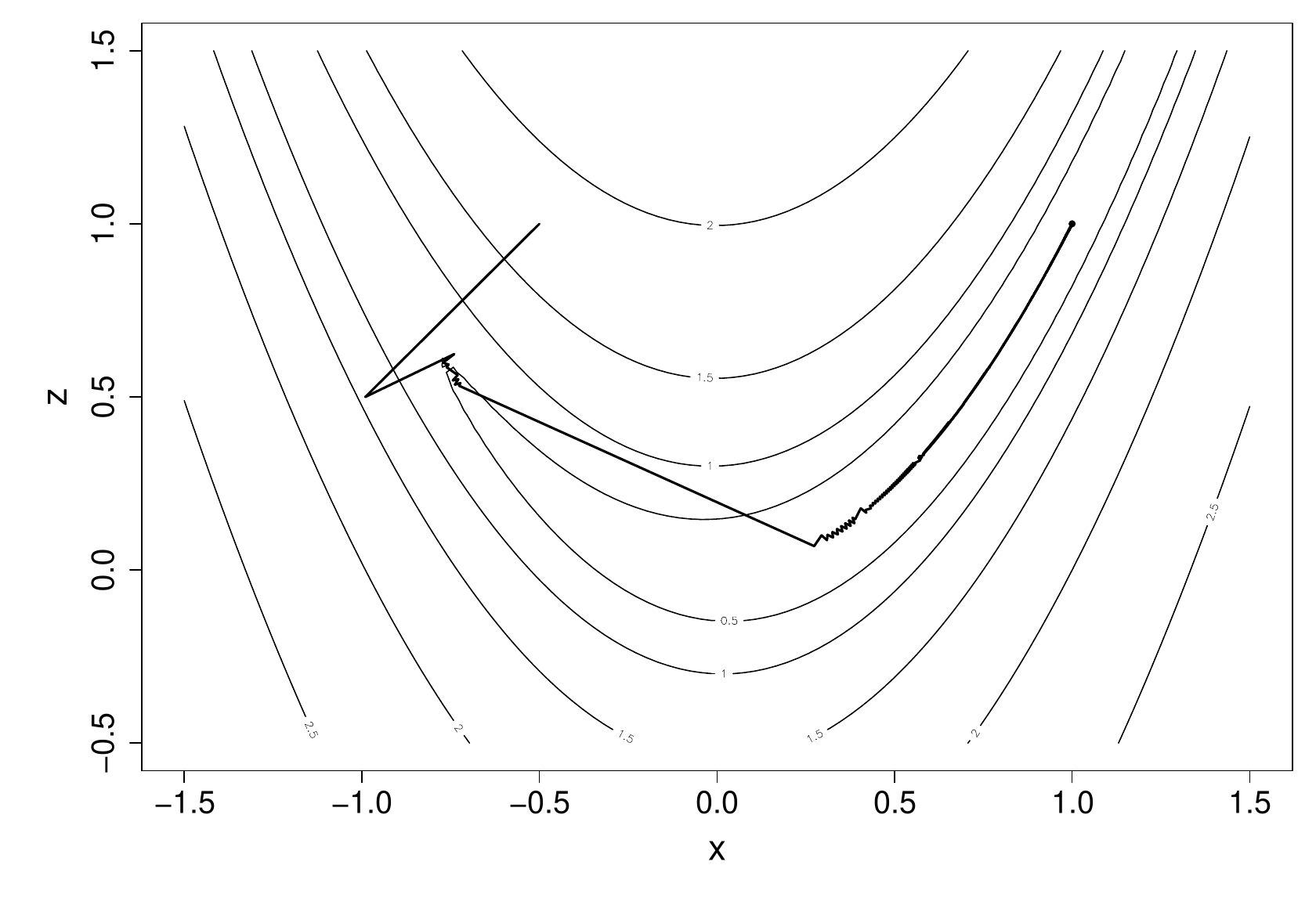
It took 14,845 steps to reach the minimum. This excruciatingly slow progress is typical of the steepest descent method. Another disadvantage of steepest descent is scale dependence: imagine linearly re-scaling so that the axis in the above plot ran from -5 to 15, but the contours were unchanged. This would change all the steepest descent directions. By contrast, the methods considered next are scale invariant.
3.4.3 Newton’s method
As steepest descent approaches the minimum, the first derivative term retained in the Taylor approximation of becomes negligible relative to the neglected second derivative term. This largely explains the method’s poor performance. Retaining the second derivative term in the Taylor expansion yields the method of choice for a wide range of problems: Newton’s method. Taylor’s theorem implies that
Differentiating the r.h.s. w.r.t. and setting the result to we have
as the equation to solve for the step which will take us to the turning point of the (quadratic) Taylor approximation of . This turning point will be a minimum (of the approximation) if is positive definite, and can also be derived directly without vector calculus by completing the square.
Notice how Newton’s method automatically suggests a search direction and a step length. Usually we simply accept the Newton step, , unless it fails to lead to sufficient decrease in . In the latter case the step length is repeatedly halved until sufficient decrease is achieved.
The second practical issue with Newton’s method is the requirement that is positive definite. There is no guarantee that it will be, especially if is far from the optimum. This would be a major problem, were it not for the fact that the solution to
is a descent direction for any positive definite . To see this, put as a search direction in our first-order approximation,
for small due to the positive-definiteness of . This gives us the freedom to modify to make it positive definite, and still be guaranteed a descent direction. One approach is to take the symmetric eigen-decomposition of , reverse the sign of any negative eigenvalues, replace any zero eigenvalues with a small positive number and then replace by the matrix with this modified eigen-decomposition. Computationally cheaper alternatives simply add a multiple of the identity matrix to , sufficiently large to make the result positive definite. Note that steepest descent corresponds to the choice , and so inflating the diagonal of the Hessian corresponds to nudging the search direction from that of the Newton method towards that of steepest descent, and this is usually a fairly safe and conservative thing to do.
Combining these steps gives a practical Newton algorithm. Starting with and a guesstimate …
-
1.
Evaluate , and , implying a quadratic approximation to , via Taylor’s theorem.
-
2.
Test whether is a minimum, and terminate if it is.
-
3.
If is not positive definite, perturb it so that it is (thereby modifying the quadratic model of ).
-
4.
The search direction is now defined by the solution to
i.e. the minimising the current quadratic model.
-
5.
If is not sufficiently lower than , repeatedly halve until it is.
-
6.
Set , increment by one and return to step 1.
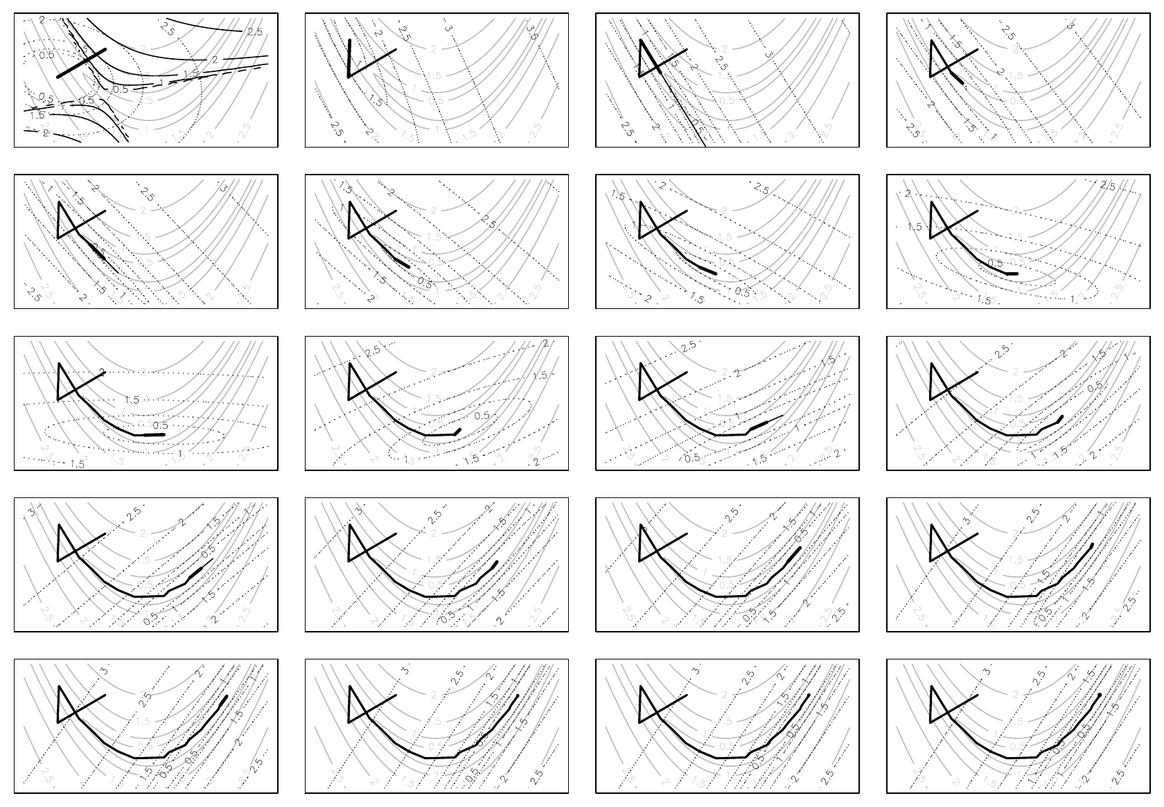
The following figure illustrates the progress of the method on Rosenbrock’s function, working across rows from top left. Grey contours show the function, dotted show the quadratic approximation at the current best point, and, if present, black contours are the quadratic approximation before modification of the Hessian. The thick black line tracks the steps accepted, while the thin black line shows any suggested steps that were reduced. Note the fact that the method converged in 20 steps, compared to the 14,845 steps taken by steepest descent.
3.4.4 Quasi-Newton methods
Newton’s method usually performs very well, especially near the optimum, but to use it we require the second derivative (Hessian) matrix of the objective. This can be tedious to obtain. Furthermore, if the dimension of is large, then solving for the Newton direction can be a substantial part of the computational burden of optimisation. Is it possible to produce methods that only require first derivative information, but with efficiency rivalling Newton’s method, rather than steepest descent?
The answer is yes. One approach is to replace the exact Hessian, of Newton’s method, with an approximate Hessian based on finite differences of gradients. The finite difference intervals must be chosen with care (see section 4.2), but the approach is reliable (recall that any positive definite matrix in place of the Hessian will yield a descent direction, so an approximate Hessian should be unproblematic). However, finite differencing for the Hessian is often more costly than exact evaluation, and there is no saving in solving for the search direction.
The second approach is to use a quasi-Newton method. The basic idea is to use first derivative information gathered from past steps of the algorithm to accumulate an approximation to the Hessian at the current best point. In principle, this approximation can be used exactly like the exact Hessian in Newton’s method, but if structured carefully, such an algorithm can also work directly on an approximation to the inverse of the Hessian, thereby reducing the cost of calculating the actual step. It is also possible to ensure that the approximate Hessian is always positive definite.
Quasi-Newton methods were invented in the mid 1950’s by W.C. Davidon (a physicist). In the mathematical equivalent of not signing the Beatles, his paper on the method was rejected (it was eventually published in 1991). There are now many varieties of Quasi-Newton method, but the most popular is the BFGS method 2 , which will be briefly covered here.
We suppose that at step we have already computed and an approximate Hessian . So, just as with a regular Newton method, we solve
to obtain a new search direction, leading either to a new directly, or more likely via line search. We now have the problem of how to appropriately update the approximate Hessian, . We want the approximate Hessian to give us a good quadratic approximation of our function about . If is our new approximate positive definite Hessian at the step, we have the function approximation
The basic requirement of a quasi Newton method is that the new Hessian should be chosen so that the approximation should exactly match — i.e. the approximation should get the gradient vector at the previous best point, , exactly right. Taking the gradient of the above approximation gives
Evaluating this at leads to our requirement
and hence
where and . The so-called secant equation (3.2) will only be feasible for positive definite under certain conditions on and , but we can always arrange for these to be met by appropriate step length selection (see Wolfe conditions, Nocedal & Wright, 2006, §3.1). Note, in particular, that pre-multiplying (3.2) by gives for positive definite Hessian, so must be positive. Still, the secant equation is under-determined, so we need to constrain the problem further in order to identify an appropriate unique solution. For quasi Newton methods, this is typically done by proposing a low-rank update to the previous Hessian. Methods exist which use a rank 1 update, but BFGS uses a rank 2 update of the form
For (good) reasons that we don’t have time to explore here, the choice , is made, and substituting this update into the secant equation allows solving for and , giving the BFGS update,
where . By substitution, we can directly verify that this satisfies the secant equation. Now let’s work in terms of the inverse approximate Hessian, , since this will allow us to avoid solving a linear system at each iteration. A naive re-write of our update would be
but this is a low-rank update of an inverse, and hence a good candidate for application of Woodbury’s formula. It is actually a bit tedious to apply Woodbury directly, but if we can guess the solution,
we can verify that it is correct by direct multiplication. We can also double-check that this update satisfies the modified secant equation, (it does). The BFGS update is usually given in the form above, but for actual implementation on a computer, it can be expanded as
and then some careful thinking about the order and re-use of computational steps within the update can lead to a very efficient algorithm.
The BFGS method then works exactly like Newton’s method, but with in place of the inverse of , and without the need for second derivative evaluation or for perturbing the Hessian to achieve positive definiteness. It also allows direct computation of the search direction via
A finite difference approximation to the Hessian is often used to start the method. The following figure illustrates its application (showing every second step of 38).
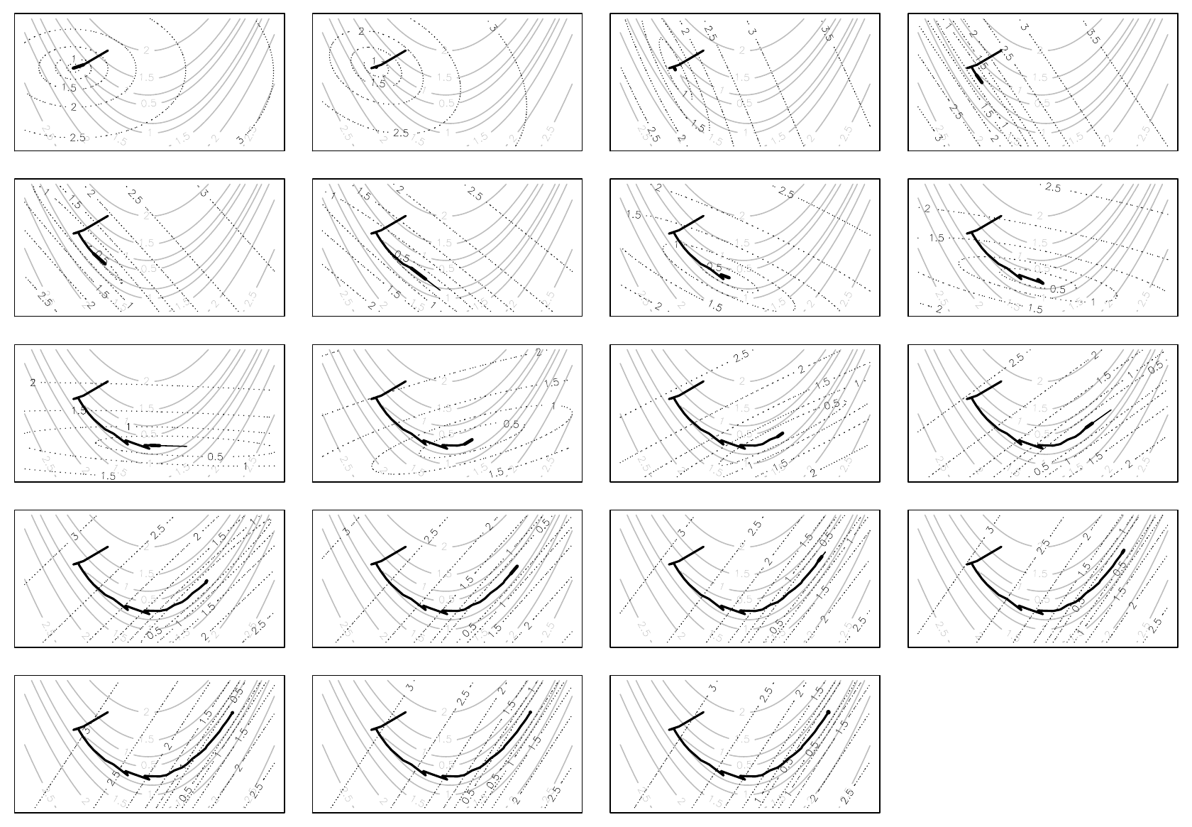
Notice how this quasi-Newton method has taken nearly twice as many steps as the Newton method, for the same problem, and shows a greater tendency to ‘zig-zag’. However, it is still computationally cheaper than finite differencing for the Hessian, which would have required an extra 20 gradient evaluations, compared to quasi-Newton. Compared to steepest descent it’s miraculous.
L-BFGS
It is also worth being aware of a variant of BFGS, known as L-BFGS, with the “L” standing for limited memory. This algorithm is mainly intended for very high-dimensional functions, where working with a full inverse Hessian would be an issue for either computational or memory reasons. Here, rather than propagating the full inverse Hessian matrix at each step, a low rank approximation of it is implicitly updated and propagated via the recent history of the process. The following Wikipedia pages provide a little additional context.
3.4.5 The Nelder–Mead polytope method
What if even gradient evaluation is too taxing, or if our objective is not smooth enough for Taylor approximations to be valid (or perhaps even possible)? What can be done with function values alone? The Nelder–Mead polytope 3 method provides a rather successful answer, and as with the other methods we have met, it is beautifully simple.
Let be the dimension of . At each stage of the method we maintain distinct vectors, defining a polytope in (e.g. for a 2-dimensional , the polytope is a triangle). The following is iterated until a minimum is reached/ the polytope collapses to a point.
-
1.
The search direction is defined as the vector from the worst point (vertex of the polytope with highest objective value) through the average of the remaining points.
-
2.
The initial step length is set to twice the distance from the worst point to the centroid of the others. If it succeeds (meaning that the new point is no longer the worst point) then a step length of 1.5 times that is tried, and the better of the two accepted.
-
3.
If the previous step did not find a successful new point then step lengths of half and one and a half times the distance from the worst point to the centroid are tried.
-
4.
If the last two steps failed to locate a successful point then the polytope is reduced in size, by linear rescaling towards the current best point (which remains fixed.)
-
5.
When a point is accepted, the current worst point is discarded, to maintain points, and the algorithm returns to step 1.
Variations are possible, in particular with regard to the step lengths and shrinkage factors.
The following figure illustrates the polytope method in action. Each polytope is plotted, with the line style cycling through, black, grey and dashed black. The worst point in each polytope is highlighted with a circle.
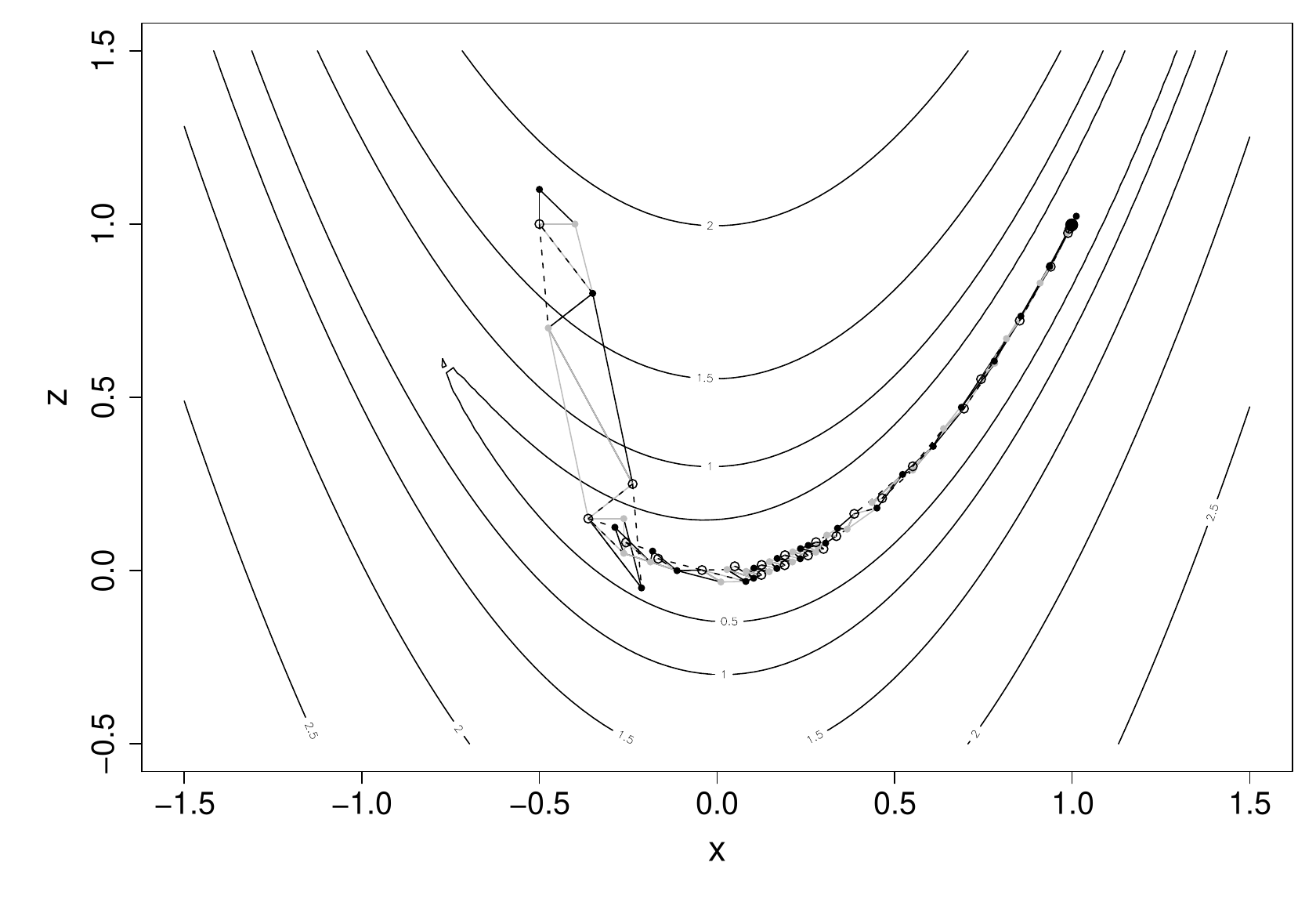
In this case it took 79 steps to reach the minimum of Rosenbrock’s function. This is somewhat more than Newton or BFGS, but given that we need no derivatives in this case, the amount of computation is actually less.
On the basis of this example you might be tempted to suppose that Nelder-Mead is all you ever need, but this is generally not the case. If you need to know the optimum very accurately then Nelder-Mead will often take a long time to get an answer that Newton based methods would give very quickly. Also, the polytope can get ‘stuck’, so that it is usually a good idea to restart the optimisation from any apparent minimum (with a new polytope having the apparent optimum as one vertex), to check that further progress is really not possible. Essentially, Nelder-Mead is good if the answer does not need to be too accurate, and derivatives are hard to come by, but you wouldn’t use it as the underlying optimiser for general purpose modelling software, for example.
3.4.6 Other methods
These notes can only provide a brief overview of some important methods. There are many other optimisation methods, and quite a few are actually useful. For example:
-
In likelihood maximisation contexts the method of scoring is often used. This replaces the Hessian in Newton’s method with the expected Hessian.
-
The Gauss-Newton method is another way of getting a Newton type method when only first derivatives are available. It is applicable when the objective is somehow related to a sum of squares of differences between some data and the model predictions of those data, and has a nice interpretation in terms of approximating linear models. It is closely related to the algorithm for fitting GLMs.
-
Conjugate gradient methods are another way of getting a good method using only first derivative information. The problem with steepest descent is that if you minimise along one steepest descent direction then the next search direction is always at right angles to it. This can mean that it takes a huge number of tiny zig-zagging steps to minimise even a perfectly quadratic function. If is the dimension of , then Conjugate Gradient methods aim to construct a set of consecutive search directions such that successively minimising along each will lead you exactly to the minimum of a quadratic function.
-
Simulated annealing is a gradient-free method for optimising difficult objectives, such as those arising in discrete optimisation problems, or with very spiky objective functions. The basic idea is to propose random changes to , always accepting a change which reduces , but also accepting moves which increase the objective, with a probability which decreases with the size of increase, and also decreases as the optimisation progresses.
-
Stochastic gradient descent (SGD) is an increasingly popular approach to optimisation of likelihoods arising from very large data sets. Each step of SGD is a gradient descent based on a new objective derived from a random subset of the data. The stochastic aspect can speed up convergence and the use of a relatively small subset of the data can speed up each iteration: https://en.wikipedia.org/wiki/Stochastic_gradient_descent
-
The EM algorithm is a useful approach to likelihood maximisation when there are missing data or random effects that are difficult to integrate out.
3.5 Constrained optimisation
Sometimes optimisation must be performed subject to constraints on . An obvious way to deal with constraints is to re-parameterise to arrive at an unconstrained problem. For example if we might choose to work in terms of the unconstrained where , and more complicated re-parameterisations can impose quite complex constraints in this way. While often effective re-parameterisation suffers from at least three problems:
-
1.
It is not possible for all constraints that might be required.
-
2.
The objective is sometimes a more awkward function of the new parameters than it was of the old.
-
3.
There can be problems with the unconstrained parameter estimates tending to . For example is above is best estimated to be zero then the best estimate of is .
A second method is to add to the objective function a penalty function penalising violation of the constraints. The strength of such a penalty has to be carefully chosen, and of course the potential to make the objective more awkward than the original applies here too.
The final set of approaches treat the constraints directly. For linear equality and inequality constraints constrained Newton type methods are based on the methods of quadratic programming. Non-linear constraints are more difficult, but can often be discretised into a set of approximate linear constraints.
3.6 Modifying the objective
If you have problems optimising an objective function, then sometimes it helps to modify the function itself. For example:
-
Reparameterisation can turn a very unpleasant function into something much easier to work with (e.g. it is often better to work with precision than with standard deviation when dealing with normal likelihoods).
-
Transform the objective. e.g. will be ‘more convex’ than : this is usually a good thing.
-
Consider perturbing the data. For example an objective based on a small sub sample of the data can sometimes be a good way of finding starting values for the full optimisation. Similarly resampling the data can provide a means for escaping small scale local minima in an objective if the re-sample based objective is alternated with the true objective as optimisation progresses, or if the objective is averaged over multiple re-samples. cf. SGD.
-
Sometimes a problem with optimisation indicates that the objective is not a sensible one. e.g. in the third example in section 3.3, an objective based on getting the observed ACF right makes more sense, and is much better behaved.
3.7 Software
R includes a routine optim for general purpose optimisation by BFGS, Nelder-Mead, Conjugate Gradient or Simulated Annealing. The R routine nlm uses Newton’s method and will use careful finite difference approximations for derivatives which you don’t supply. R has a number of add on packages e.g. quadprog, linprog, trust to name but 3. See http://neos-guide.org/ for a really useful guide to what is more generally available.
Should you ever implement your own optimisation code? Many people reply with a stern ‘no’, but I am less sure. For the methods presented in detail above, the advantages of using your own implementation are (i) the un-rivalled access to diagnostic information and (ii) the knowledge of exactly what the routine is doing. However, if you do go down this route it is very important to read further about step length selection and termination criteria. Where greater caution is needed is if you require constrained optimisation, large scale optimisation or to optimise based on approximate derivatives. All these areas require careful treatment.
3.8 Further reading on optimisation
-
Nocedal and Wright (2006) Numerical Optimization 2nd ed. Springer, is a very clear and up to date text. If you are only going to look at one text, then this is probably the one to go for.
-
Gill, P.E. , W. Murray and M.H. Wright (1981) Practical Optimization Academic Press, is a classic, particularly on constrained optimisation. I’ve used it to successfully implement quadratic programming routines.
-
Dennis, J.E. and R.B. Schnabel (1983) Numerical Methods for Unconstrained Optimization and Nonlinear Equations (re-published by SIAM, 1996), is a widely used monograph on unconstrained methods (the nlm routine in R is based on this one).
-
Press WH, SA Teukolsky, WT Vetterling and BP Flannery (2007) Numerical Recipes (3rd ed.), Cambridge and Monahan, JF (2001) Numerical Methods of Statistics, Cambridge, both discuss Optimization at a more introductory level.
- Computer scientists have an interesting classification of the ‘difficulty’ of problems that one might solve by computer. If is the problem ‘size’ then the easiest problems can be solved in polynomial time: they require operations where is finite. These problems are in the P-class. Then there are problems for which a proposed solution can be checked in polynomial time, the NP class. NP-complete problems are problems in NP which are at least as hard as all other problems in NP in a defined sense. NP hard problems are at least as hard as all problems in NP, but are not in NP: so you can’t even check the answer to an NP hard problem in polynomial time. No one knows if P and NP are the same, but if any NP-complete problem turned out to be in P, then they would be.
- BFGS is named after Broyden, Fletcher, Goldfarb and Shanno all of whom independently discovered and published it, around 1970. Big Friendly Giant Steps is the way all Roald Dahl readers remember the name, of course (M.V.Bravington, pers. com.).
- This is also known as the downhill simplex method, which should not be confused with the completely different simplex method of linear programming.