MATH4341 - Spatio-temporal statistics

Term 2: Temporal modelling and time series analysis

Term 2, Lab 4 (and practice test)

Overview

This lab document is an R Markdown file. It should be downloaded to your computer, and then loaded up into RStudio. Follow the instructions provided, writing code to solve the required problems into the provided code blocks, as directed. Regularly check on progress by “knitting” the document to a PDF and checking that the output is correct. You may find it helpful to have a separate R session window for writing, testing and debugging code solutions, before pasting back into the markdown document - that is up to you. But do make sure that all of your solutions are in this markdown document and that the document compiles into a PDF correctly.

This practical is constructed in a similar way to the practical test that will take place in week 10 (although this practical is shorter, to fit into a 50 minute session). At the end of the real test in week 10, you will compile your completed document to a PDF file and upload the PDF file (only) to Gradescope for marking. For this practical, you should make sure that you are able to compile your document to a PDF, but you don’t need to upload anything anywhere at the end of the session. You should simply check later that your completed PDF looks similar to the solution file that will be provided after the session.

Note that whilst the week 10 test will be conducted under exam conditions, during this lab it’s fine to discuss with your neighbours or ask for my help if you get stuck.

The dataset

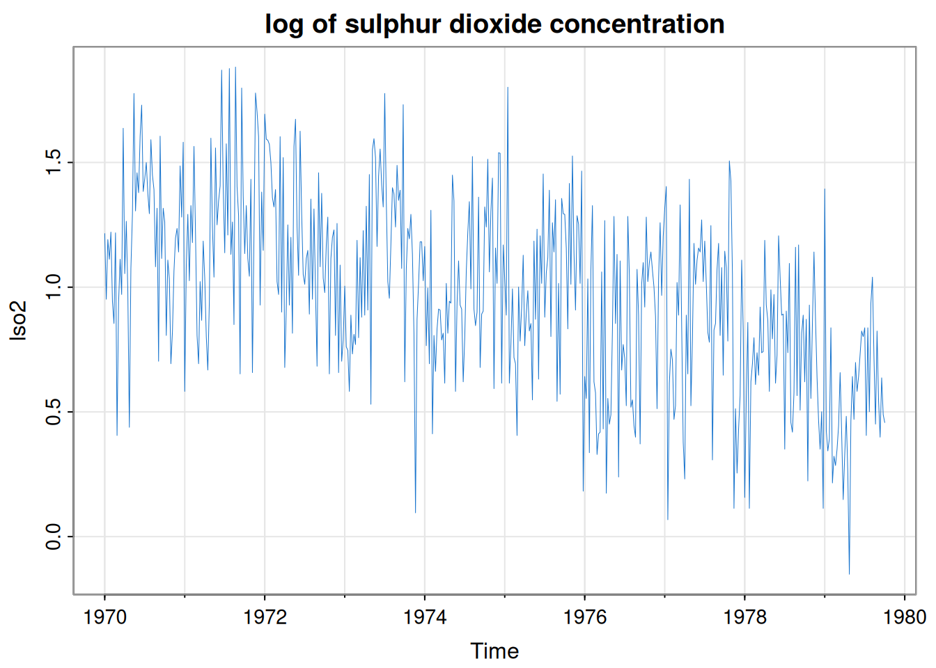
The following code block loads up the required library and plots the dataset that is to be the subject of our analysis.

library(astsa) # required library
lso2 = log(so2) # log of the SO2 data (the log is more Gaussian)
tsp(lso2) # start, end, frequency
[1] 1970.00 1979.75   52.00
n = length(lso2)
n
[1] 508
tsplot(lso2, col=4, lwd=0.5,
    main="log of sulphur dioxide concentration")

The dataset is weekly (frequency 52) data.

Smoothing

We will begin with some simple smoothing of the time series data to reveal possible overall trends and seasonality. Compute a 12-week moving average of the data, and overlay it onto the plot below with a red line of thickness 2. You might want to consult Chapter 1 of the notes.

tsplot(lso2, col=4, lwd=0.5,
    main="log of sulphur dioxide concentration")

## YOUR CODE HERE:

This hints at a gradual downward trend with some annual seasonality.

A different way to smooth the data is to just keep the low frequency coefficients from a DFT and zero out the rest. Produce a smoothing of the data in this way by just keeping the first 15 DFT frequency components. Again, overlay the smooth on the plot below using a red line of thickness 2. You might want to consult Chapter 5 of the notes.

tsplot(lso2, col=4, lwd=0.5,
    main="log of sulphur dioxide concentration")

## An inverse FFT function is likely to be useful
ifft = function(x) fft(x, inverse=TRUE) / length(x)
## YOUR CODE HERE:

ARMA fitting and forecasting

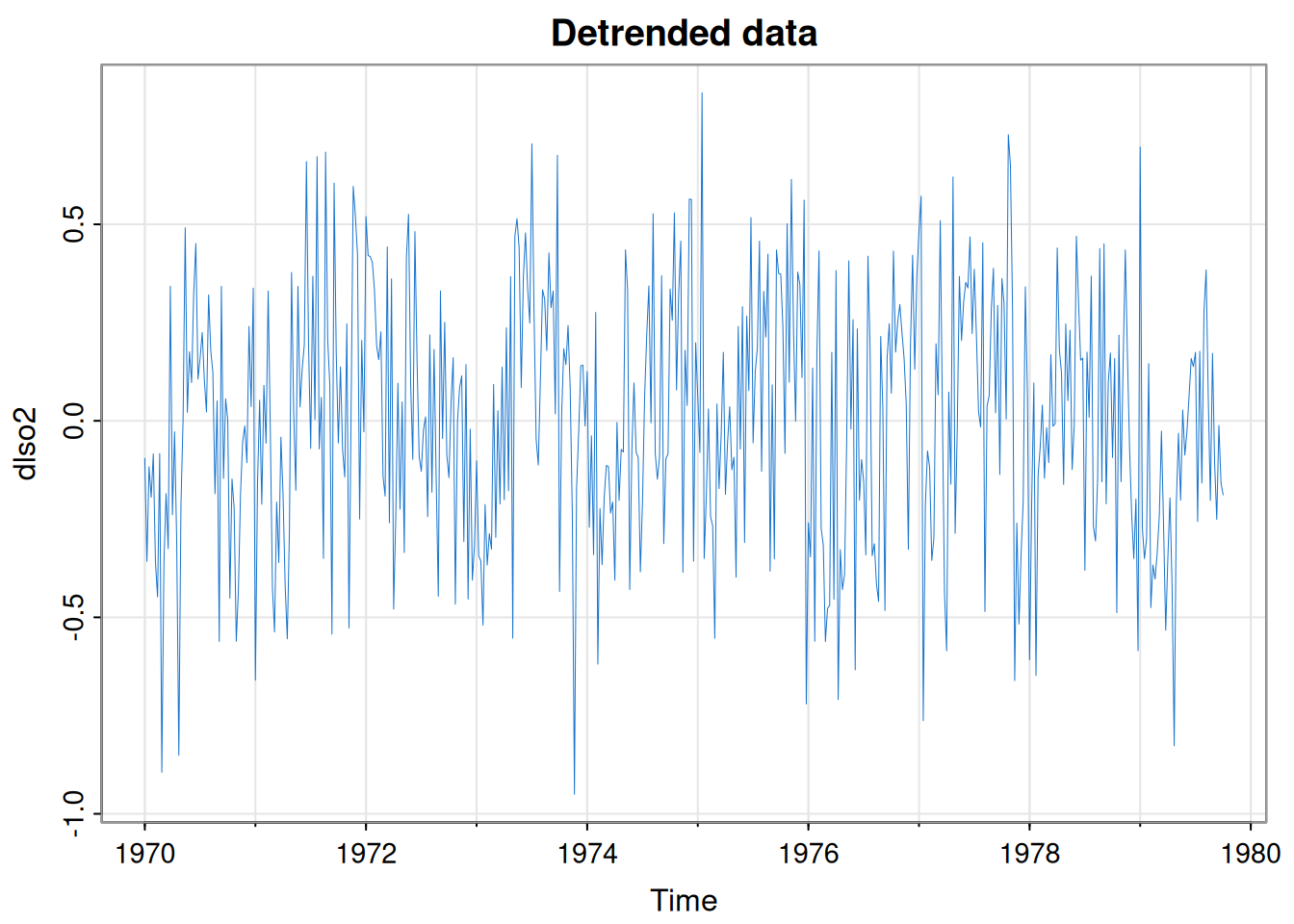
We will now turn our attention to ARMA modelling, and for this we will want to focus mainly on the detrended data.

dlso2 = detrend(lso2)
tsplot(dlso2, col=4, lwd=0.5, main="Detrended data")

Plot the ACF and PACF of the detrended data, and on the basis of this, fit an appropriate auto-regressive model (using the arima function). You might want to consult Chapter 4 of the notes.

## YOUR CODE HERE:

In order to understand the nature of the fitted auto-regressive model, produce an appropriately smoothed periodogram of the detrended data, and overlay on top the spectrum of the fitted model (with a thicker line). Note that you may need to divide the spectrum of the fitted model by the frequency of the time series in order to put it on the same scale as the periodogram spectrum (due to the way the spectral density is often defined for frequencies other than one).

## YOUR CODE HERE:

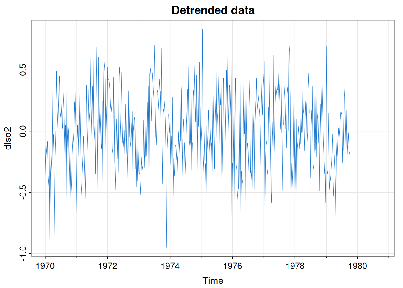
We now want to forecast the detrended data. Add one year (52 weeks) of forecasts to the plot below (in red), together with upper and lower 2 standard deviation intervals.

tsplot(dlso2, col=4, lwd=0.5, main="Detrended data",
       xlim=c(tsp(dlso2)[1], tsp(dlso2)[2]+1))

## YOUR CODE HERE:

Of course we are really more interested in the non-detrended data (shown below). First, add a linear trend line to the plot (in green), and then, by adding the linear trend to the forecasts you computed above, add appropriate forecasts and upper and lower intervals (in red) to the plot below. You may ignore the uncertainty in your regression line.

tsplot(lso2, col=4, lwd=0.5, main="log SO2 concentration",
       xlim=c(tsp(dlso2)[1], tsp(dlso2)[2]+1))

## YOUR CODE HERE:

The end

The practical is now complete. If you have completed all of the code blocks as required, you should check that you can compile this completed file into a PDF file, and that the PDF file looks correct. That is all you need to do. You don’t need to upload it anywhere. After the summative test in Week 10 (which will be constructed in a similar way to this lab), you will then upload your compiled PDF file (only) to Gradescope for marking, before the deadline.