1 Introduction to time series
1.1 Time series data
1.1.1 What is a time series?
A time series is simply a collection of observations indexed by time. Since we measure time in a strictly ordered fashion, from the past, through the present, to the future, we assume that our time index is some subset of the real numbers, and in many cases, this subset will be a subset of the integers. So, for example, we could denote the observation at time \(t\) by \(x_t\). Then our time series could be written \[ \mathbf{x} = (x_1, x_2, \ldots, x_n) \] if we have \(n\) observations corresponding to time indices \(t=1,2,\ldots,n\).
When we use (consecutive) integers for the time index, we are implicitly assuming that the observations are equispaced in time.
Crucially, in time series analysis, the order of the observations matters. If we permute our observations in some way, the time series is different. Statistical models for time series are not invariant to permutations of the data. This is obviously different to many statistical models you have studied previously, where observations (within some subgroup) are iid (or exchangeable).
In the second half of this module we will study spatial statistical models and the analysis of spatial data. Spatial data is indexed by a position in space, and the spatial index is often assumed to be a subset of \(\mathbb{R}^2\) or \(\mathbb{R}^3\). Spatial models also have the property that they are not invariant to a permutation of the observations. Indeed, there is a strong analogy to be drawn between time series data and 1-d spatial data, where the spatial index is a subset of \(\mathbb{R}\). This analogy can sometimes be helpful, and there are situations where it makes sense to treat time series data as 1-d spatial data.
However, the very special nature of the 1-d case (in particular, the complete ordering property of the reals), and the strong emphasis in classical time series analysis on the case of equispaced observations, means that models for time series and methods for the analysis of time series data typically look very different to the models used in spatial statistics.
We will therefore temporarily forget about spatial modelling and spatial statistics, and develop models and methods explicitly focused on time series. We will better understand the relationships between time series and spatial analysis much later, towards the end of Term 2.
1.1.2 An example
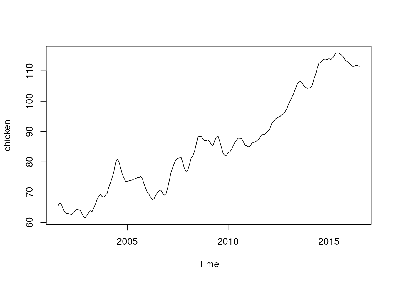
Consider the price of chicken in the US (measured in US cents per pound in weight of chicken). This is a dataset in the R CRAN package astsa.
Note that observations close together in time are more highly correlated than observations at disparate times. This uses the R base function for plotting time series (plot.ts, since the chicken data is a ts object). We could also plot using tsplot from the astsa package.
tsplot(chicken)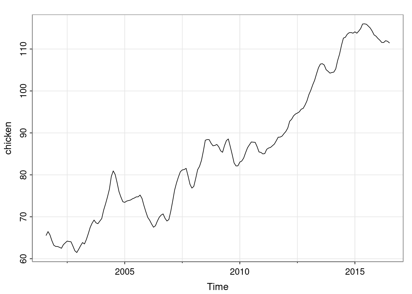
If we wanted, we could make it look a bit nicer.
tsplot(chicken, col=4, lwd=2,
  main="Price of chicken", ylab="US cents per pound")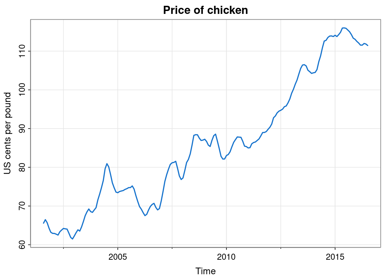
Remember that you can get help on the astsa package with help(package="astsa"), and help on particular functions with (eg.) ?tsplot. You can get a list of datasets in the package with data(package="astsa"). Note that there is also an online guide to this package: fun with astsa.
1.1.3 Detrending
It is clear that observations close together in time are more highly correlated than observations far apart, but is that simply because of the slowly increasing trend? We can see by detrending the data in some way. There are many ways one can detrend a time series, but here, since there looks to be a roughly linear increase in price with time, we could detrend by fitting a linear regression model using time as a covariate, and subtracting off the linear fit, in order to leave us with some detrended residuals.
We could do this with base R functions.
tc = time(chicken)
res = residuals(lm(chicken ~ tc))
dc = ts(res, start=start(chicken), freq=frequency(chicken))
plot(dc, lwd=2, col=4, main="Detrended price of chicken")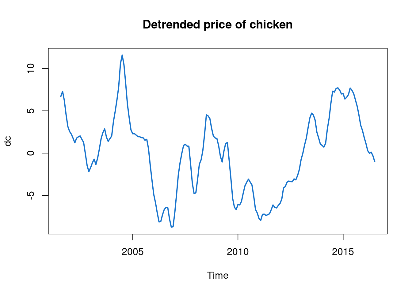
But the astsa package has a built-in detrend function which makes this much easier.
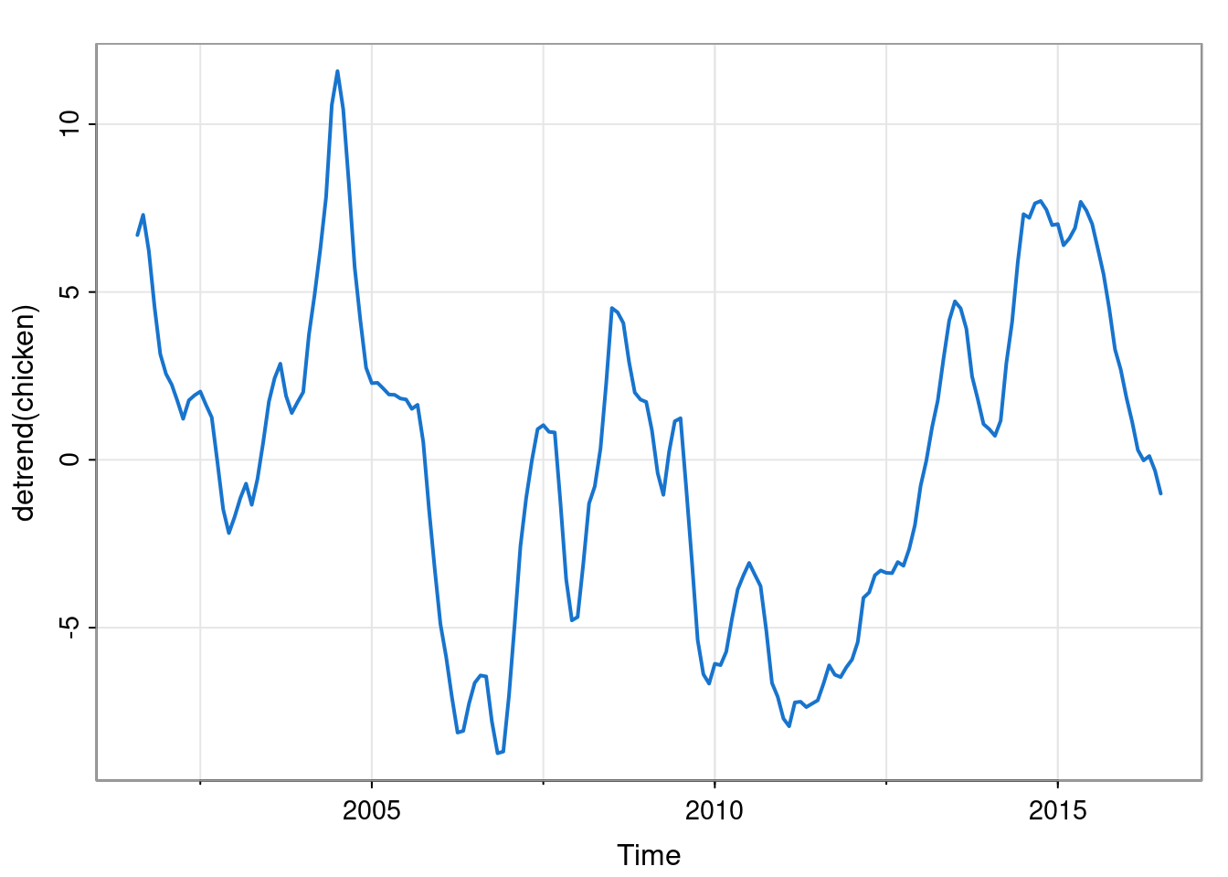
Note that despite having removed the obvious trend from the data it is still the case that observations close together in time are more highly correlated than observations far apart. We can visualise this nearby correlation more clearly by producing a scatter plot showing each observation against the previous observation.
lag1.plot(dc, pch=19, col=4)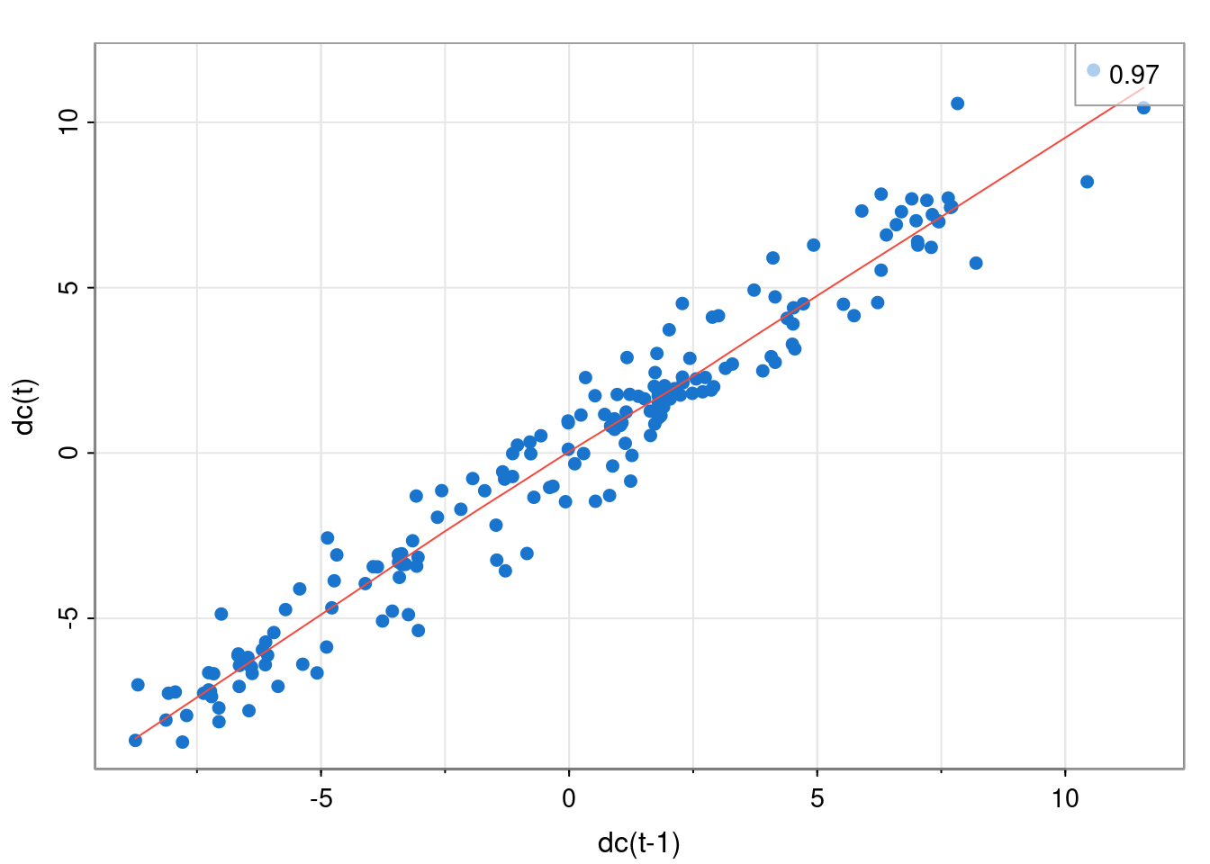
For iid observations, there would be no correlation between adjacent values. Here we see that the correlation at lag 1 (observations one time index apart) is around 0.97. This correlation decreases as the lag increases.
acf1(dc)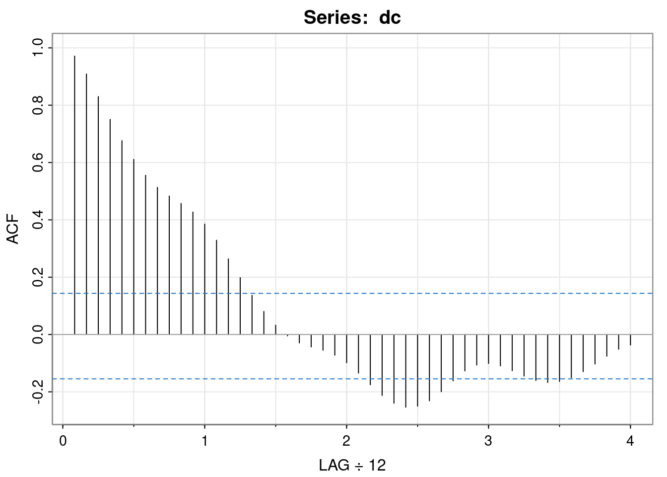
 [1]  0.97  0.91  0.83  0.75  0.68  0.61  0.56  0.51  0.48  0.46  0.43  0.39
[13]  0.33  0.26  0.20  0.14  0.08  0.03  0.00 -0.03 -0.04 -0.05 -0.07 -0.10
[25] -0.13 -0.18 -0.21 -0.24 -0.25 -0.25 -0.23 -0.20 -0.16 -0.13 -0.11 -0.10
[37] -0.11 -0.13 -0.14 -0.16 -0.17 -0.16 -0.15 -0.13 -0.10 -0.08 -0.05 -0.04
This plot of the auto-correlation against lag is known as the auto-correlation function (ACF), or sometimes correlogram, and is an important way to understand the dependency structure of a (stationary) time series. From this plot we see that observations have to be more than one year apart for the auto-correlations to become statistically insignificant.
1.2 Filtering time series
1.2.1 Smoothing with convolutional linear filters
Sometimes short-term fluctuations in a time series can obscure longer-term trends. We know that the sample mean has much lower variance than an individual observation, so some kind of (weighted) average might be a good way of getting rid of noise in the data. However, for time series models, it only really makes sense to perform an average locally. This is the idea behind linear filters.
By way of example, consider the chicken price data, and consider forming a new time series where each new observation is the sample mean of the 25 observations closest to that time point.
tsplot(chicken, col=4,
  main="Chicken price smoothed with a moving average filter")
lines(filter(chicken, rep(1/25, 25)), col=2, lwd=2)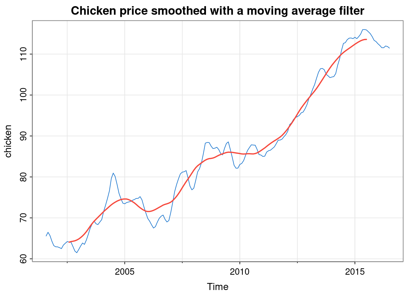
Note that the new time series is shorter than the original time series, and some convention is required for aligning the two time series. Here, R’s filter function has done something sensible. We see that the filter has done exactly what we wanted - it has smoothed out short-term fluctuations, better revealing the long-term trend in the data.
A convolutional linear filter defines a new time series \(\mathbf{y}=\{y_t\}\) from an input time series \(\mathbf{x}=\{x_t\}\) via \[ y_t = \sum_{i=q_1}^{q_2} w_i x_{t-i}, \] for \(q_1 \leq 0 \leq q_2\) and pre-specified weights, \(w_{q_1},\ldots,w_{q_2}\) (so \(q_2-q_1+1\) weights in total). If the weights are non-negative and sum to one, then the filter represents a moving average, but this is not required. Note that if the input series is defined for time indices \(1, 2, \ldots, n\), then the output series will be defined for time indices \(q_2+1, q_2+2, \ldots, n+q_1\), and hence will be of length \(n+q_1-q_2\).
In the context of digital signal processing (DSP), this would be called a finite impulse response (FIR) filter, and the convolution operation is sometimes summarised with the shorthand notation \[ \mathbf{y} = \mathbf{w} * \mathbf{x}. \]
Very commonly, a symmetric filter will be used, where \(q_1=-q\) and \(q_2=q\), for some \(q>0\), and \(w_i=w_{-i}\). Although the weight vector is of length \(2q+1\), there are only \(q+1\) free parameters to be specified. In this case, if the input time indices are \(1,2,\ldots,n\), then the output indices will be \(q+1,q+2,\ldots,n-q\) and hence the output will be of length \(n-2q\).
1.2.2 Seasonality
Let’s look now at the quarterly share earnings for the company Johnson and Johnson.
tsplot(jj, col=4, lwd=2, main="Quarterly J&J earnings")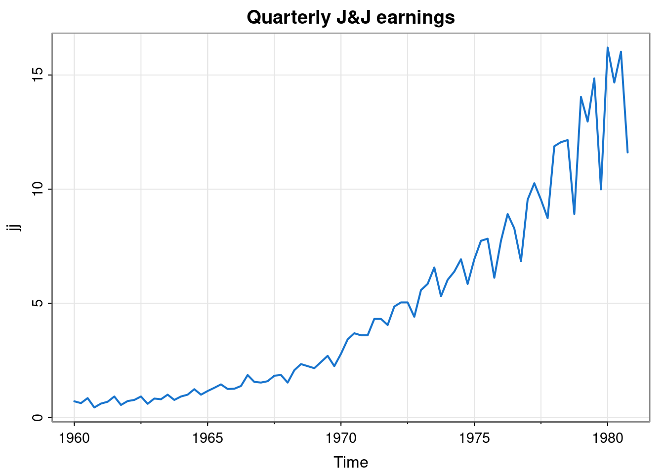
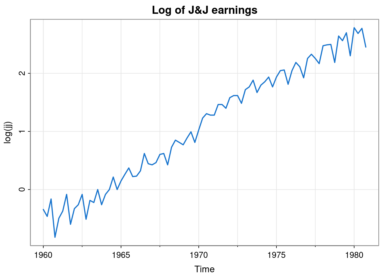
We can see an exponential increase in the overall trend. We can also see that the deviations from the overall trend seem to exhibit a regular pattern with a period of 4. There seem to be particular quarters where earnings are lower than the overall trend, and others where they seem to be higher. This kind of seasonality in time series data is very common. Seasonality can happen on many time scales, but yearly, weekly and daily is most common. On closer inspection, we see that the seasonal effects seem to be increasing exponentially, in line with the overall trend. We could attempt to develop a multiplicative model for this data, but it might be simpler to just take logs.
To progress further, we probably want to detrend in some way. We could take out a linear fit, but we could also estimate the trend by smoothing out the seasonal effects with a moving average that averages over 4 consecutive quarters to give a yearly average. That is, we could apply a convolutional linear filter with weight vector \[ \mathbf{w} = (0.25, 0.25, 0.25, 0.25). \] The problem with this is that it is of even length, so it represents an average that lies between two quarters, and so doesn’t align nicely with our existing series. We can fix this by using a symmetric moving average centred on a given quarter by instead using a weight vector of length 5. \[ \mathbf{w} = (0.125, 0.25, 0.25, 0.25, 0.125). \] Now each quarter still receives a total weight of 0.25, but the weight for the quarter furthest away is split across two different years.
sjj = filter(log(jj), c(0.125,0.25,0.25,0.25,0.125))
tsplot(sjj, col=4, lwd=2, main="Smoothed log of J&J earnings")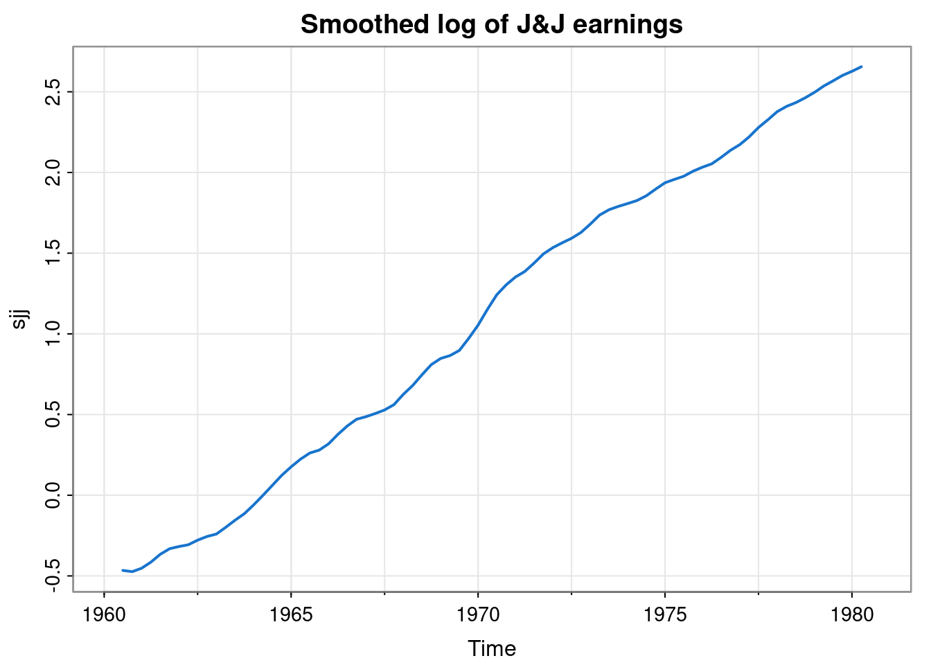
We can see that this has nicely smoothed out the seasonal fluctuations giving just the long term trend.
So, in general, when trying to deseasonalise a time series with seasonal fluctuations with period \(m\), if \(m\) is odd (which is quite rare), then just use a filter with a weight vector of length \(m\), with all weights set to \(1/m\). In the more typical case where \(m\) is even, use a weight vector of length \(m+1\) where the end weights are set to \(1/(2m)\) and all other weights are set to \(1/m\).
This deseasonalisation process is an example of what DSP people would call a low-pass filter. It has filtered out the high-frequency oscillations, allowing the long term (low frequency) behaviour to pass through.
We can now detrend the log data by subtracting off this trend to leave just the seasonal effects.
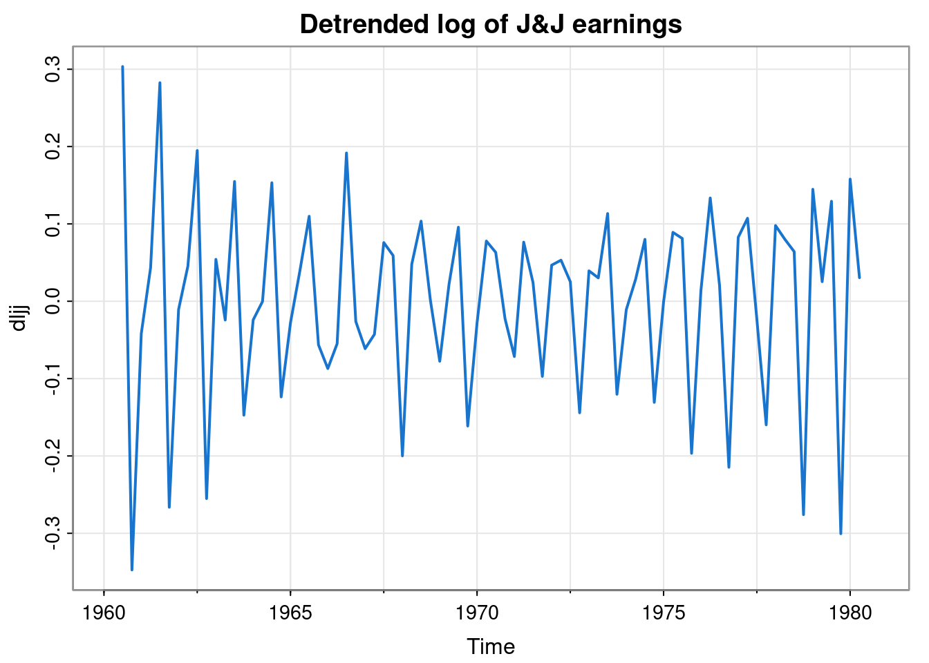
Note that we could have directly computed the detrended data by applying a convolutional linear filter with weight vector \[ \mathbf{w} = (-0.125,-0.25,0.75,-0.25,-0.125) \]
dljj = filter(log(jj), c(-0.125,-0.25,0.75,-0.25,-0.125))
tsplot(dljj, col=4, lwd=2, main="Detrended log of J&J earnings")
Note that this filter has weights summing to zero. This detrending process is an example of what DSP people would call a high-pass filter. It has allowed the high frequency oscillations to pass through, while removing the long term (low frequency) behaviour.
We could use this detrended data to get a simple estimate of the seasonal effects associated with each of the four quarters.
[1] -0.0001916332 0.0403896607 0.1121470367 -0.1492881658We can now strip out these seasonal effects.
dsdtljj = dljj - seff
tsplot(dsdtljj, col=4, lwd=2,
  main="Detrended and deseasonalised log of J&J earnings")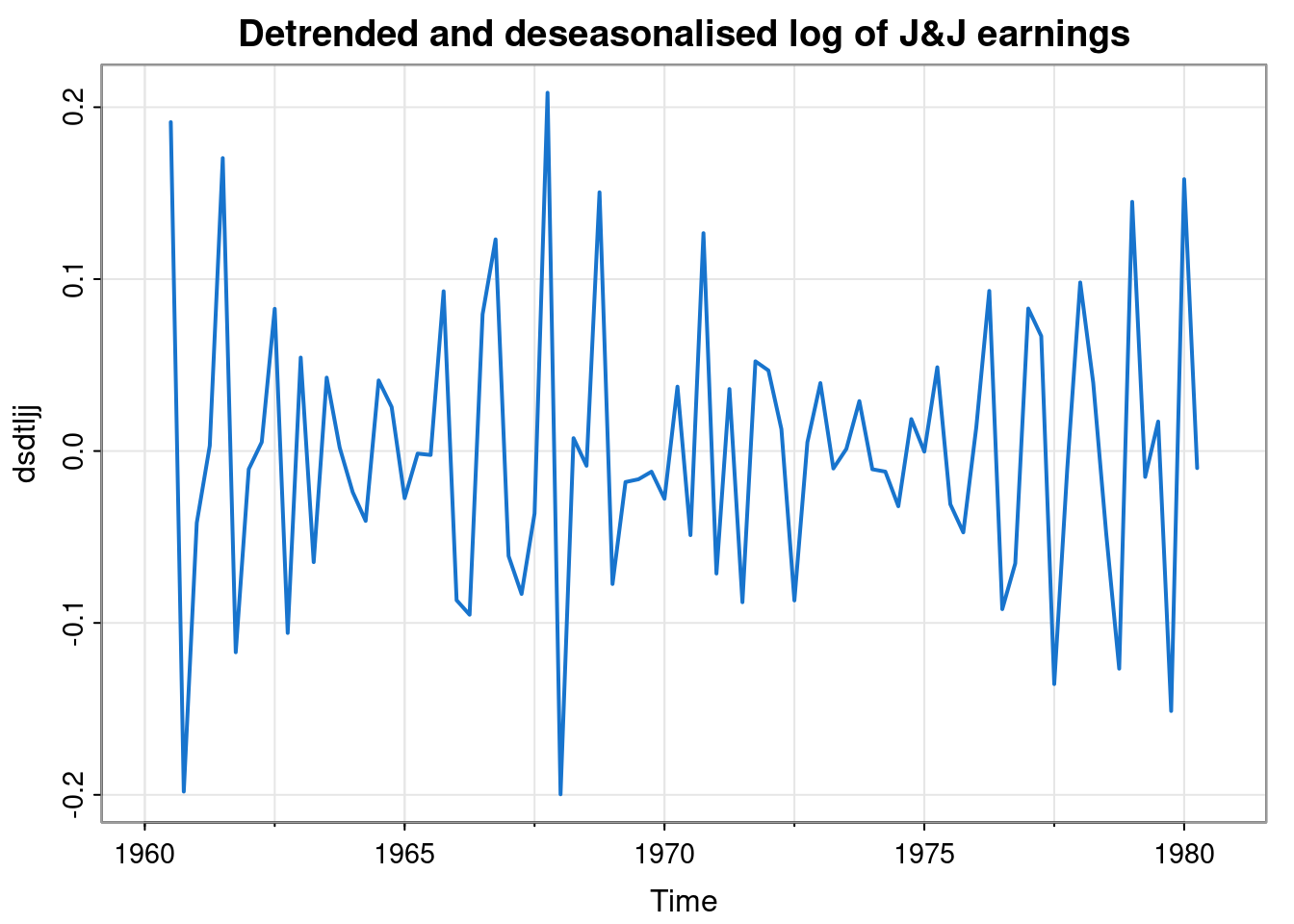
Not perfect (as the seasonal effects aren’t perfectly additive), and definitely lots of auto-correlation left, but it’s getting closer to some kind of correlated noise process.
1.2.3 Exponential smoothing and auto-regressive linear filters
We previously smoothed the chicken price data by applying a moving average filter to it. That is by no means the only way we could smooth the data. One drawback of the moving average filter is that you lose values at each end of the series. Losing values at the right-hand end is particularly problematic if you are using historic data up to the present in order to better understand the present (and possibly forecast into the future). In the on-line context it makes sense to keep a current estimate of the underlying level (smoothed value), and update this estimate with each new observation. Exponential smoothing is probably the simplest variant of this approach. We can define a smoothed time series \(\mathbf{s}=\{s_t\}\) using the input time series \(\mathbf{x}=\{x_t\}\) via the update equation \[ s_t = \alpha x_t + (1-\alpha)s_{t-1}, \] for some fixed \(\alpha\in[0,1]\). It is clear from this definition that the new smoothed value is a weighted average of the current observation and the previous smoothed value. High values of \(\alpha\) put more weight on the current observation (and hence, less smoothing), whereas low values of \(\alpha\) put less weight on the current observation, leading to more smoothing. It is called exponential smoothing because recursive application of the update formula makes it clear that the weights associated with observations from the past decay away exponentially with time. It is worth noting that the update relation can be re-written \[ s_t = s_{t-1} + \alpha(x_t - s_{t-1}), \] which can sometimes be convenient.
Note that some strategy is required for initialising the smoothed state. eg. if the first observation is \(x_1\), then to compute \(s_1\), some initial \(s_0\) is required. Sometimes \(s_0=0\) is used, but more often \(s_0 = x_1\) is used, which obviously involves looking ahead at the data, but ensures that \(s_1 = x_1\), which is often sensible.
The smoothing value, \(\alpha\) can be specified subjectively, noting that this is no more subjective than choosing the size of the smoothing window for a moving average filter. Alternatively, some kind of cross-validation strategy can be used, based on, say, one-step ahead prediction errors.
The stats::filter function is not flexible enough to allow us to implement this kind of linear filter, so we instead using the signal::filter function.
alpha = 0.1
sm = signal::filter(alpha, c(1, alpha-1), chicken, init.y=chicken[1])
tsp(sm) = tsp(chicken)
tsplot(chicken, col=4)
lines(sm, col=2, lwd=2)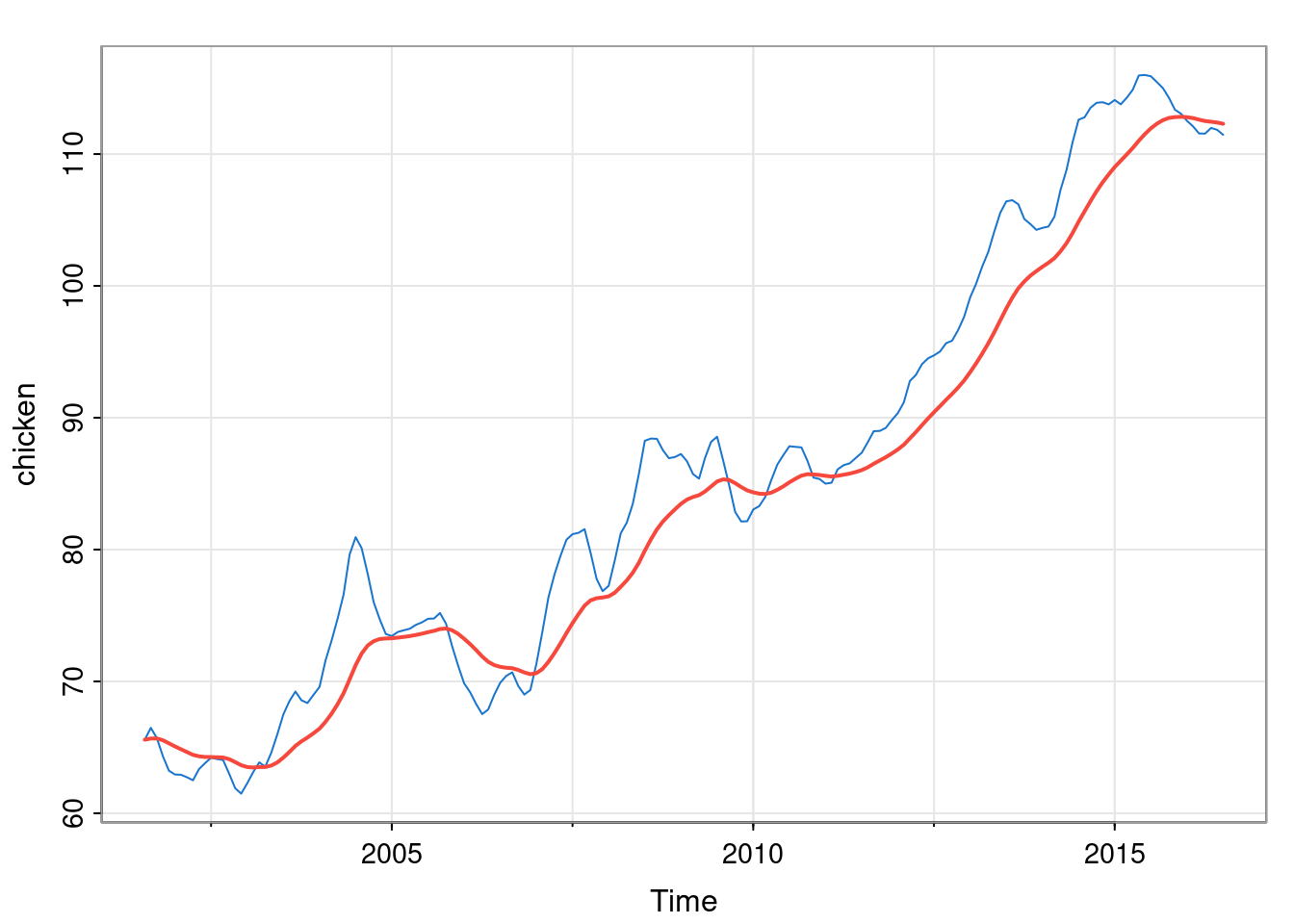
We will figure out the details of the signal::filter function shortly. We see that the filtered output is much smoother than the input, but also that it somewhat lags the input series. This can be tuned by adjusting the smoothing parameter. Less smoothing will lead to less lag.
Exponential smoothing is a special case of an auto-regressive moving average (ARMA) linear filter, which DSP people would call an infinite impulse response (IIR) filter. The ARMA filter relates an input time series \(\mathbf{x}=\{x_t\}\) to an output time series \(\mathbf{y}=\{y_t\}\) via the relation \[ \sum_{i=0}^p a_i y_{t-i} = \sum_{j=0}^q b_j x_{t-j}, \] for some vectors \(\mathbf{a}\) and \(\mathbf{b}\), of length \(p+1\) and \(q+1\), respectively. This can obviously be rearranged as \[ y_t = \frac{1}{a_0}\left(\sum_{j=0}^q b_j x_{t-j} - \sum_{i=1}^p a_i y_{t-i}\right). \] These are more powerful than the convolution filters considered earlier, since they allow the propagation of persistent state information.
It is clear that if we choose \(\mathbf{a}=(1, \alpha-1)\), \(\mathbf{b}=(\alpha)\) we get the exponential smoothing model previously described. The signal::filter function takes \(\mathbf{b}\) and \(\mathbf{a}\) as its first two arguments, which should explain the above code block.
1.3 Multivariate time series
The climhyd dataset records monthly observations on several variables relating to Lake Shasta in California (see ?climhyd for further details). The monthly observations are stored as rows of a data frame. We can get some basic information about the dataset as follows.
str(climhyd)'data.frame': 454 obs. of 6 variables:
$ Temp : num 5.94 8.61 12.28 11.61 20.28 ...
$ DewPt : num 1.436 -0.285 0.857 2.696 5.7 ...
$ CldCvr: num 0.58 0.47 0.49 0.65 0.33 0.28 0.11 0.08 0.15 0.27 ...
$ WndSpd: num 1.22 1.15 1.34 1.15 1.26 ...
$ Precip: num 160.53 65.79 24.13 178.82 2.29 ...
$ Inflow: num 156 168 173 273 233 ...head(climhyd) Temp DewPt CldCvr WndSpd Precip Inflow
1 5.94 1.436366 0.58 1.219485 160.528 156.1173
2 8.61 -0.284660 0.47 1.148620 65.786 167.7455
3 12.28 0.856728 0.49 1.338430 24.130 173.1567
4 11.61 2.696482 0.65 1.147778 178.816 273.1516
5 20.28 5.699536 0.33 1.256730 2.286 233.4852
6 23.83 8.275339 0.28 1.104325 0.508 128.4859We can then plot the observations.
tsplot(climhyd, ncol=2, col=2:7)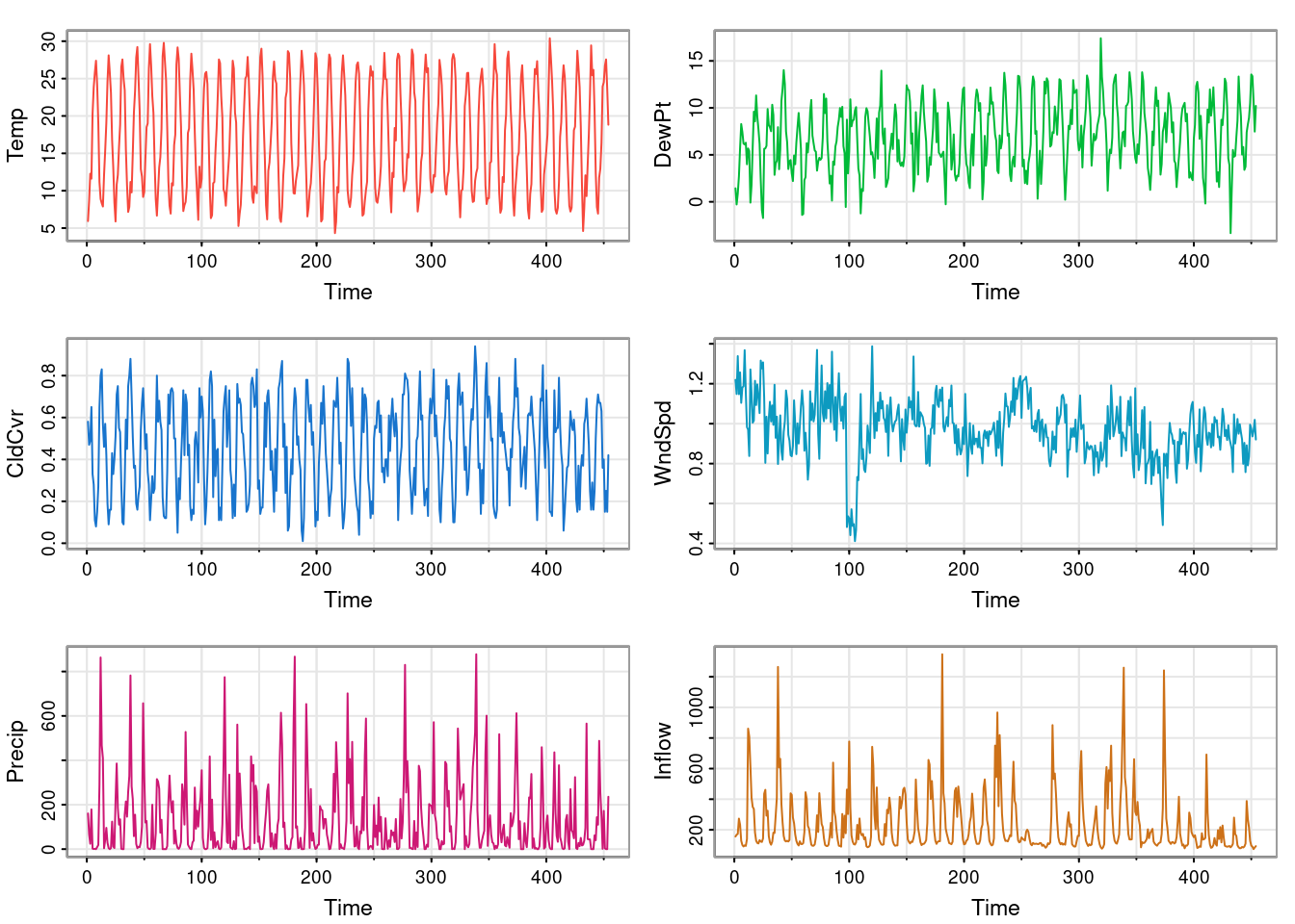
The data can be regarded as a collection of six univariate time series. We could just treat them completely separately, applying univariate time series analysis techniques to each variable in turn. However, this wouldn’t necessarily be a good idea unless the series are all independent of one another. But typically, the reason we study a collection of time series together is because we suspect that they are not all independent of one another. Here, we could look at a simple pairs plot of the variables.
pairs(climhyd, col=4, pch=19, cex=0.5)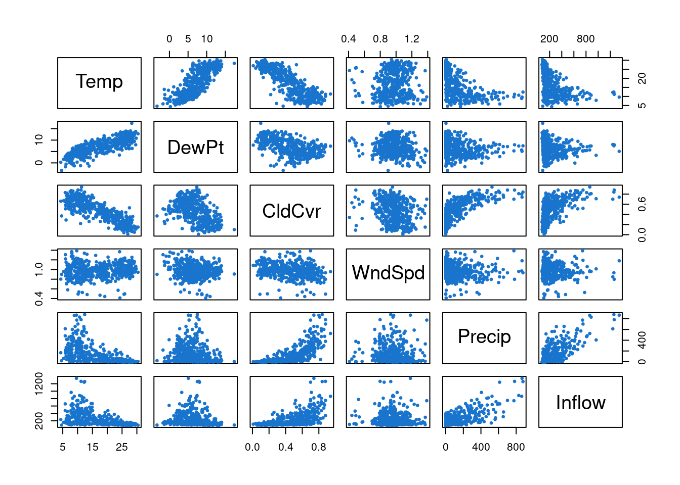
We see that there do appear to be cross-correlations between the series, strongly suggesting that the component series are not independent of one another. It is then an interesting question as to the best way to analyse a collection of dependent time series, with correlations across variables as well as over time. We will come back to this question later.
1.4 Time series analysis
We’ve looked at some basic exploratory tools for visualising and decomposing time series into trend, seasonal and residual components. But we know from previous courses that to do any meaningful statistical inference for the underlying features, or probabilistic prediction (or forecasting), then it is very helpful to have a statistical model of the data generating process. We typically approach this by building a model with some systematic components (such as a trend and seasonal effects), and then using an appropriate probability model for the residuals. But in most simple statistical models, this residual process is assumed to be iid. However, we have seen that for time series, it is often implausible that the residuals will be iid. We have seen that it is likely that we should be able to account for systematic effects, leaving residuals that are mean zero. In many cases, it may even be plausible that the residuals have constant variance. But we have seen that typically the residuals will be auto-correlated, with correlations tailing off as the lag increases. It would therefore be useful to have a family of discrete time stochastic processes that can model this kind of behaviour. It will turn out that ARMA models are a good solution to this problem, and we will study these properly in Chapter 3. But first we will set the scene by examining a variety of (first and second order) linear Markovian dynamical systems. This will help to provide some context for ARMA models, and hopefully make them seem a bit less mysterious.