4 Estimation and forecasting
In this chapter we consider the problem of fitting time series models to observed time series data, and using the fitted models to forecast the unobserved future observations of the time series.
4.1 Fitting ARMA models to data
Since we mainly know about ARMA models, we concentrate here on the problem of fitting ARMA models to time series data. We assume that the time series has been detrended and has zero mean, so that fitting a mean zero stationary model to the data makes sense. We will also assume that the order of the process (the values of \(p\) and \(q\)) are known. This is unlikely to be true in practice, but the idea is that appropriate values can be identified by looking at ACF and PACF plots for the (detrended) time series.
4.1.1 Moment matching
Since we have seen how to compute the ACF of ARMA models, and we know how to compute the empirical ACF of an observed time series, it is natural to consider estimating the parameters of an ARMA model by finding parameters that match up well with the empirical ACF. Since the ACF encodes the second moments of the time series, this is moment matching, or the method of moments in the context of stationary time series analysis. This approach works best in the context of AR(p) models, so we focus mainly on that case.
4.1.1.1 AR(p)
Recall that the Yule-Walker equations from Section 3.2.1 could be written in either auto-covariance or auto-correlation form. We start with the auto-covariance form. If we define \(\pmb{\gamma}=(\gamma_1,\ldots,\gamma_p)^\top\), \(\pmb{\phi}=(\phi_1,\ldots,\phi_p)^\top\) and let \(\mathsf{\Gamma}\) be the \(p\times p\) symmetric matrix \[ \mathsf{\Gamma} = \{\gamma_{i-j}|i,j=1,\ldots,p\}, \] then the Yule-Walker equations can be written in matrix form as \[ \mathsf{\Gamma}\pmb{\phi} = \pmb{\gamma},\quad\sigma^2 = \gamma_0-\pmb{\phi}^\top\pmb{\gamma}. \] Then given an empirical estimate of the auto-covariance function computed from time series data, we can construct estimates \(\hat\gamma_0\), \(\hat{\pmb{\gamma}}\), and hence \(\hat{\mathsf{\Gamma}}\), and use them to estimate the parameters of the AR(p) model as \[ \hat{\pmb{\phi}} = \hat{\mathsf{\Gamma}}^{-1}\hat{\pmb{\gamma}},\quad\hat{\sigma}^2 = \hat{\gamma}_0-\hat{\pmb{\gamma}}^\top\hat{\mathsf{\Gamma}}^{-1}\hat{\pmb{\gamma}}. \] These estimates are known as the Yule-Walker estimators of the AR(p) model parameters.
If we prefer, we can re-write all of the above in auto-correlation form. Define \(\pmb{\rho}=(\rho_1,\ldots,\rho_p)^\top\) and let \(\mathsf{P}\) be the \(p\times p\) symmetric matrix \[ \mathsf{P} = \{\rho_{i-j}|i,j=1,\ldots,p\}. \] Then the Yule-Walker equations can be written \[ \mathsf{P}\pmb{\phi} = \pmb{\rho},\quad \sigma^2 = \gamma_0(1-\pmb{\phi}^\top\pmb{\rho}). \] So, given empirical ACF estimates \(\hat{\pmb{\rho}}\), \(\hat{\mathsf{P}}\), along with an estimate of the stationary variance, \(\hat v = \hat{\gamma}_0\), we can compute parameter estimates \[ \hat{\pmb{\phi}} = \hat{\mathsf{P}}^{-1}\hat{\pmb{\rho}},\quad \hat\sigma^2 = \hat\gamma_0(1-\hat{\pmb{\rho}}^\top\hat{\mathsf{P}}^{-1}\hat{\pmb{\rho}}). \]
4.1.1.1.1 Example: AR(2)
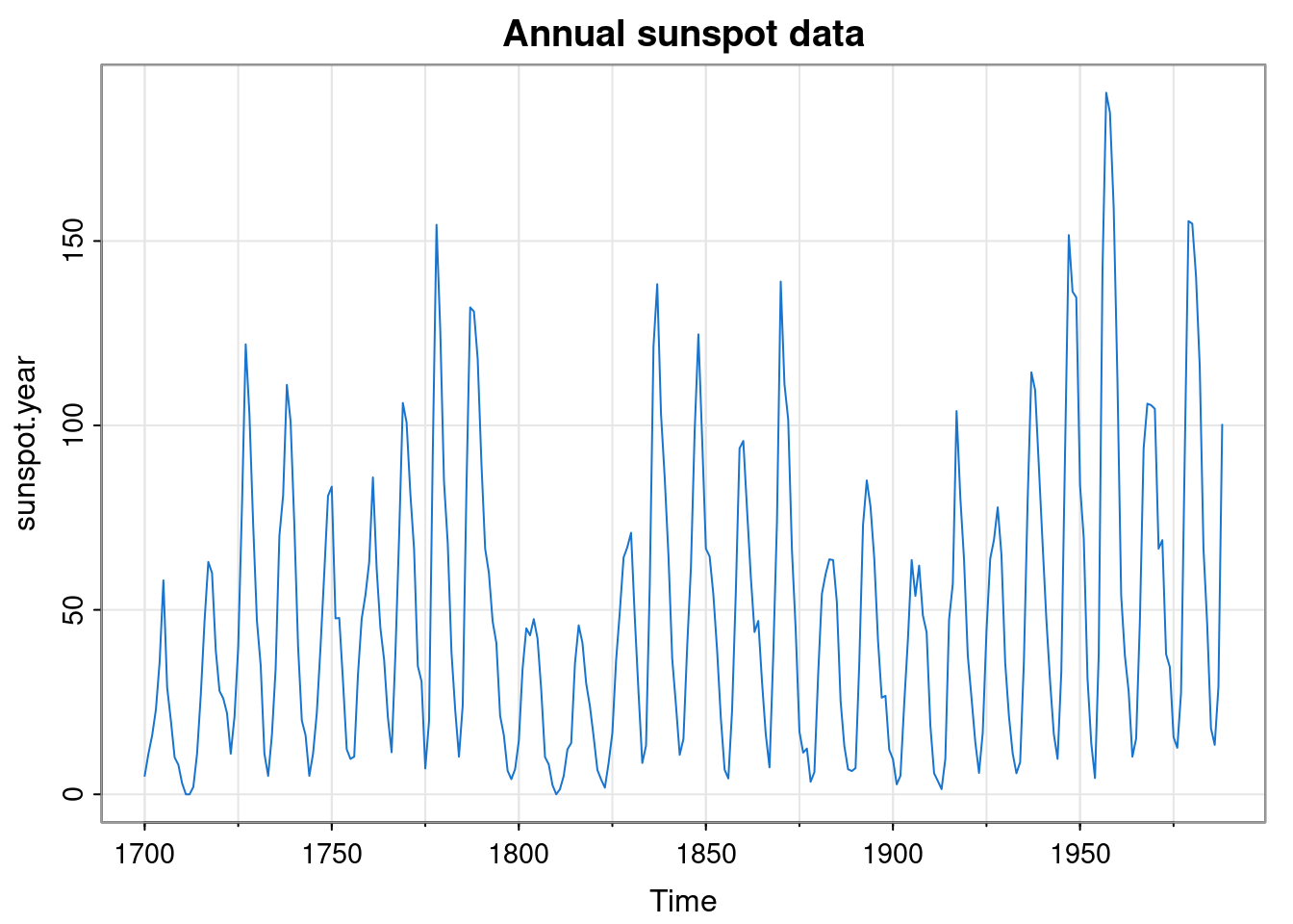
Let’s look at some of the sunspot data built in to R (?sunspot.year).
Since it is count data, it is a bit right-skewed, so the square root is a bit more Gaussian.
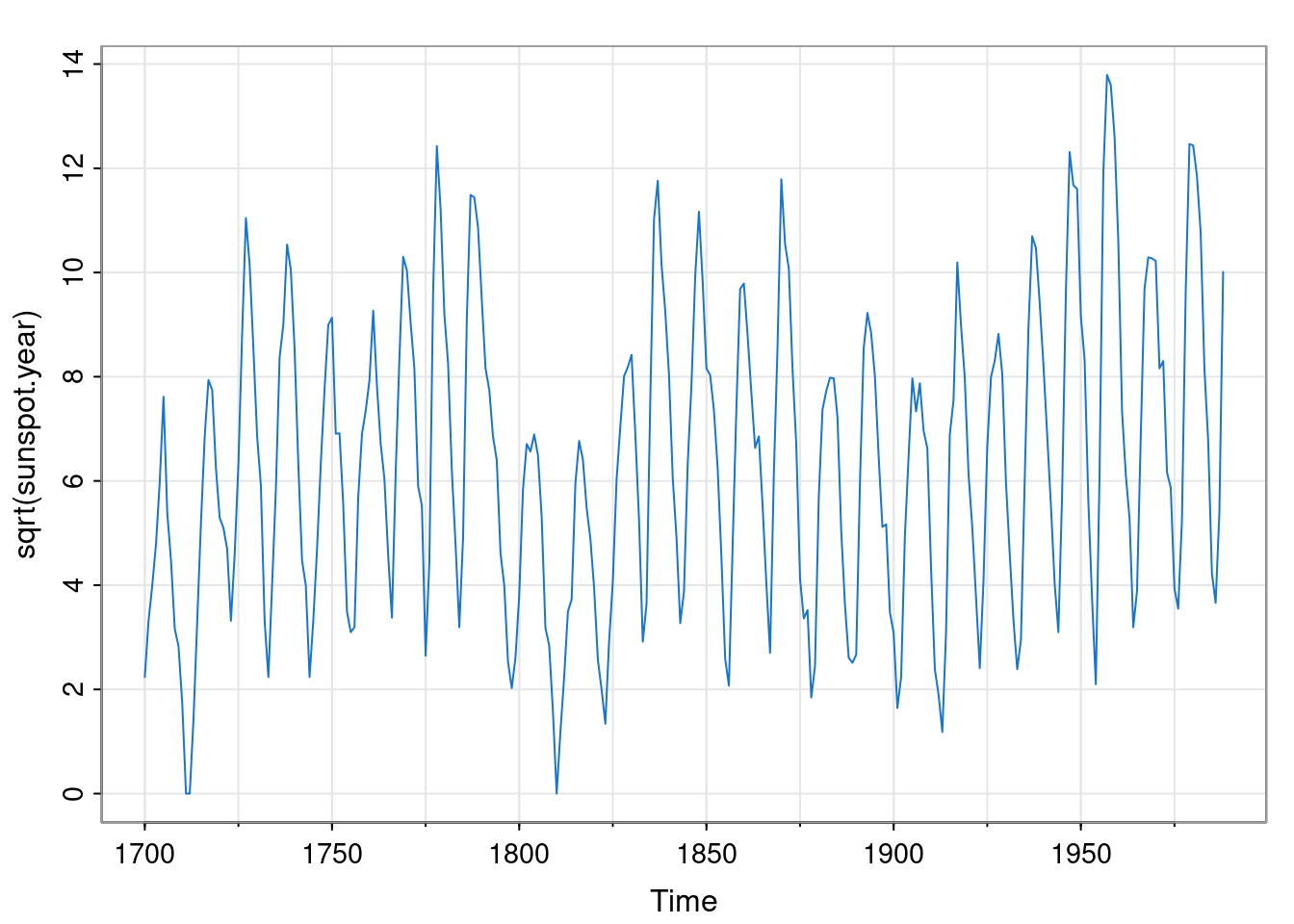
and we should detrend before fitting an ARMA model.
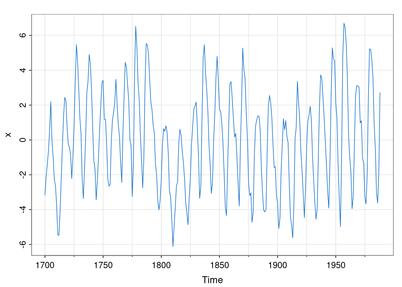
We can see some periodicity to this data, further revealed by looking at the ACF
acf2(x)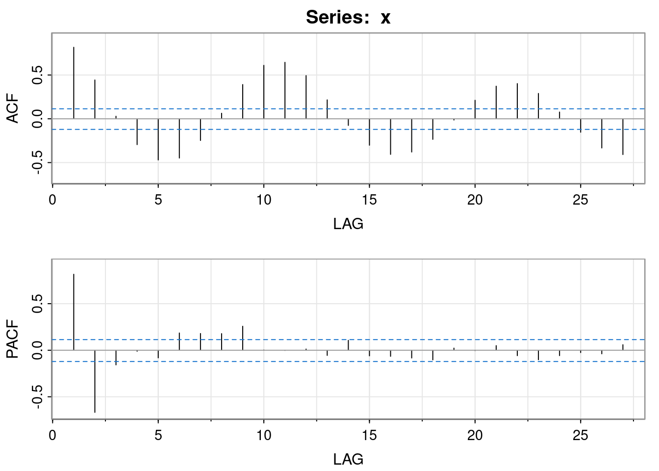
     [,1]  [,2]  [,3]  [,4]  [,5]  [,6]  [,7] [,8] [,9] [,10] [,11] [,12] [,13]
ACF  0.82  0.44  0.03 -0.29 -0.47 -0.45 -0.25 0.06 0.39  0.61  0.64  0.49  0.22
PACF 0.82 -0.67 -0.16 -0.01 -0.08  0.19  0.18 0.18 0.26  0.00  0.00  0.01 -0.06
     [,14] [,15] [,16] [,17] [,18] [,19] [,20] [,21] [,22] [,23] [,24] [,25]
ACF  -0.08 -0.30 -0.41 -0.38 -0.23 -0.01  0.21  0.37  0.40  0.29  0.08 -0.15
PACF  0.11 -0.06 -0.07 -0.08 -0.10  0.02  0.00  0.05 -0.06 -0.10 -0.06 -0.02
     [,26] [,27]
ACF  -0.33 -0.41
PACF -0.04  0.06
The ACF suggests a period of between 10 and 11 years. The PACF suggests that something like an AR(2) may be appropriate for this data, so that is what we will fit.
rho = acf(x, plot=FALSE, lag.max=2)$acf[2:3]
P = matrix(c(1, rho[1], rho[1], 1), ncol=2)
phi = solve(P, rho)
phi
[1] 1.3602493 -0.6671228These coefficients correspond to complex roots of the characteristic polynomial, as we might expect given the oscillatory nature of the data. We can confirm the suggested period of the oscillations.
So the period of the oscillations is a little under 11 years.
4.1.1.2 MA and ARMA models
We can imagine doing a similar moment matching approach for an MA\((q)\) process (or a more general ARMA model), but it doesn’t work out so nicely, due to the ACF being non-linear in the parameters. We could investigate this in more detail, but moment matching isn’t such a great parameter estimation strategy in general, so let’s just move on.
4.1.2 Least squares
As an alternative to moment matching, we can approach parameter estimation as a least squares problem, where we try to find the parameters that minimise the sum of squares of the noise terms, \(\varepsilon_t\). Again this is simpler in the case of an AR\((p)\) model, so we begin with that.
4.1.2.1 AR(p)
The model \[ x_t = \sum_{k=1}^p \phi_k x_{t-k} + \varepsilon_t,\quad t=1,2,\ldots,n \] is actually in the form of a multiple linear regression model. We can therefore treat it as a linear least squares problem, choosing parameters \(\pmb{\phi}\) to minimise \(\mathcal{L}(\pmb{\phi}) = \sum_{t=1}^n \varepsilon_t^2\). We can simplify the problem by ignoring the initialisation problem by conditioning on the first \(p\) observations and ignoring their contribution to the loss function. This gives us a so-called conditional least squares problem. We can write the model in matrix form as \[ \begin{pmatrix}x_{p+1}\\x_{p+2}\\\vdots\\x_n\end{pmatrix} = \begin{pmatrix} x_p&x_{p-1}&\cdots&x_1\\ x_{p+1}&x_{p}&\cdots&x_2\\ \vdots&\vdots&\ddots&\vdots\\ x_{n-1}&x_{n-2}&\cdots&x_{n-p} \end{pmatrix} \begin{pmatrix}\phi_1\\\phi_2\\\vdots\\\phi_p\end{pmatrix} + \begin{pmatrix}\varepsilon_{p+1}\\\varepsilon_{p+2}\\\vdots\\\varepsilon_{n}\end{pmatrix}, \] or \[ \mathbf{x} = \mathsf{X}\pmb{\phi} + \pmb{\varepsilon}, \] for appropriately defined \((n-p)\)-vectors \(\mathbf{x}\) and \(\pmb{\varepsilon}\) and \((n-p)\times p\) matrix, \(\mathsf{X}\). We then know from basic least squares theory that \[ \mathcal{L}(\pmb{\phi}) = \sum_{t=p+1}^n \varepsilon_t^2 = \Vert \pmb{\varepsilon}\Vert^2 = \pmb{\varepsilon}^\top\pmb{\varepsilon} \] is minimised by choosing \(\pmb{\phi}\) to be the solution of the normal equations, \[ \mathsf{X}^\top\mathsf{X} \pmb{\phi} = \mathsf{X}^\top\mathbf{x}, \] in other words \[ \hat{\pmb{\phi}} = (\mathsf{X}^\top\mathsf{X})^{-1}\mathsf{X}^\top\mathbf{x}. \] We can then estimate \(\sigma\) as the empirical variance of the residuals.
4.1.2.1.1 Example: AR(2)
Let us now fit the sunspot data example again, but this time using least squares.
Call:
lm(formula = xp ~ 0 + X)

Coefficients:
     X1       X2
 1.4032  -0.7086
We use R’s lm function to solve the least squares problem. Note that the coefficients are similar, but not identical, to those obtained earlier.
4.1.2.1.2 Connection between moment matching and least squares
It is clear from the definition of the matrix \(\mathsf{X}\), that its associated sample covariance matrix, \(\mathsf{X}^\top\mathsf{X}/(n-p)\) will be (unbiased and) consistent for \(\mathsf{\Gamma}\) (recall that there are \(n-p\) rows in \(\mathsf{X}\)). Then by considering a single column of the covariance matrix, similar reasoning reveals that \(\mathsf{X}^\top\mathbf{x}/(n-p)\) will be consistent for \(\pmb{\gamma}\). So if we wanted, we could use the finite sample estimates: \[ \hat{\mathsf{\Gamma}} = \frac{\mathsf{X}^\top\mathsf{X}}{n-p},\quad \hat{\pmb{\gamma}} = \frac{\mathsf{X}^\top\mathbf{x}}{n-p}. \] But if we do this, we find that our moment matching estimator, \[ \hat{\pmb{\phi}} = \hat{\mathsf{\Gamma}}^{-1}\hat{\pmb{\gamma}} = (\mathsf{X}^\top\mathsf{X})^{-1}\mathsf{X}^\top\mathbf{x} \] is just the least squares estimator. So the two approaches are asymptotically equivalent. This is the real reason why moment matching actually works quite well for AR models.
4.1.2.2 ARMA(p,q)
The approach for a general ARMA model is similar to that for an AR model, but with an extra twist. Again, the problem simplifies if we ignore the contribution associated with the first \(p\) observations. But now we also have an issue with initialising the errors. Again, we can simplify by conditioning on the first \(q\) required errors. But here we don’t actually know what to condition on, so we just condition on them all being zero. This conditional least squares approach is again approximate, but has negligible impact when \(n\) is large. We can then use the least squares loss function \[ \mathcal{L}(\pmb{\phi},\pmb{\theta}) = \sum_{t=p+1}^n \varepsilon_t^2\quad\text{where}\quad \varepsilon_t = x_t - \sum_{j=1}^p \phi_j x_{t-j} - \sum_{k=1}^q \theta_k \varepsilon_{t-k}, \] and we assume \(\varepsilon_t=0,\ \forall t\leq p\). For \(q>0\) this is a nonlinear least squares problem, so we need to minimise it numerically. There are efficient ways to do this, but the details are not especially relevant to this course.
4.1.2.2.1 Example: ARMA(2, 1)
Just for fun, let’s fit an ARMA(2, 1) to the sunspot data.
loss = function(param) {
  phi = param[1:2]; theta = param[3]
  eps = signal::filter(c(1, -phi), c(1, theta),
    x[3:length(x)], init.x=x[1:2], init.y=c(0))
  sum(eps*eps)
}

optim(rep(0.1,3), loss)$par
[1] 1.4840176 -0.7749327 -0.1623121The first two elements of the parameter vector correspond to \(\pmb{\phi}\), and the last corresponds to \(\theta\). In practice, we will typically use the built-in function arima to fit ARMA models to data.
Call:
arima(x = x, order = c(2, 0, 1), include.mean = FALSE)

Coefficients:
         ar1      ar2      ma1
      1.4828  -0.7733  -0.1631
s.e.  0.0516   0.0465   0.0785

sigma^2 estimated as 1.331:  log likelihood = -452.69,  aic = 913.39
The arima function fits using the method of maximum likelihood, considered next.
4.1.3 Maximum likelihood
Neither moment matching nor least squares are particularly principled estimation methods, so we next turn our attention to the method of maximum likelihood. As usual, the AR case is simpler, so we begin with that.
4.1.3.1 AR(p)
We can always write the likelihood function of any model as a recursive factorisation of the joint distribution of the data. So, for an AR model we could write \[\begin{align*} L(\pmb{\phi},\sigma;\mathbf{x}) &= f(\mathbf{x}) \\ &= f(x_1)f(x_2|x_1)\cdots f(x_n|x_1,\ldots,x_{n-1}) \end{align*}\] In other words, \[ L(\pmb{\phi},\sigma;\mathbf{x}) = f(x_1)\prod_{t=2}^n f(x_t|x_1,\ldots,x_{t-1}) \tag{4.1}\] This holds for any model, but for an AR\((p)\), \(X_t\) depends only on the previous \(p\) values, so we can write this as \[ L(\pmb{\phi},\sigma;\mathbf{x}) = f(x_1,\ldots,x_p)\prod_{t=p+1}^n f(x_t|x_{t-1},\ldots,x_{t-p}), \] where \(f(x_1,\ldots,x_p)\) is the joint (MVN) distribution of \(p\) consecutive observations, and \[ f(x_t|x_{t-1},\ldots,x_{t-p}) = \mathcal{N}\left(x_t;\sum_{k=1}^p\phi_k x_{t-k},\sigma^2\right), \] the normal density function. We could directly maximise this likelihood using iterative numerical methods (see below). However, the likelihood obviously simplifies significantly if we ignore the contribution of the first \(p\) observations, leading to the conditional log-likelihood \[\begin{align*} \ell(\pmb{\phi},\sigma;\mathbf{x}) &= -(n-p)\log \sigma - \frac{1}{2\sigma^2}\sum_{t=p+1}^n\left(x_t - \sum_{k=1}^p\phi_kx_{t-k}\right)^2 \\ &= -(n-p)\log \sigma - \frac{1}{2\sigma^2}\sum_{t=p+1}^n\varepsilon_t^2 . \end{align*}\] We can immediately see that as a function of \(\pmb{\phi}\), maximising this leads to exactly the least squares problem that we have already considered, and so our MLE can be obtained by solving the normal equations. The effect of conditioning on the first \(p\) observations will be negligible for long time series, but if we’d rather do exact MLE fitting using the unconditional likelihood, we just include the joint density of the first \(p\) observations and numerically maximise (possibly using the conditional fit as an initial guess). Recall that (assuming we are in the stationary regime) the joint density of the first \(p\) observations will be \(\mathcal{N}(\mathbf{0},\mathsf{V})\), where \(\mathsf{V}\) is the stationary variance matrix obtained by solving the relevant discrete Lyapunov equation.
4.1.3.1.1 Example: AR(2) MLE
Let us define and optimise the (exact) log likelihood for an AR(2) fitted to the sunspot data.
ll = function(param) {
  phi = param[1:2]; sig = param[3]
  eps = filter(x, c(1, -phi))[2:(length(x)-1)]
  V = netcontrol::dlyap(matrix(c(phi[1], phi[2], 1, 0), ncol=2),
    matrix(c(sig*sig, 0, 0, 0), ncol=2))
  (mvtnorm::dmvnorm(x[1:2], c(0, 0), V, log=TRUE)
    - (length(x)-2)*log(sig)
    - sum(eps*eps)/(2*sig*sig)
    )
  }

optim(c(1.0, -0.2, 1.0), ll, control=list(fnscale=-1))$par
[1] 1.4016403 -0.7067519 1.1619802This fit is very similar to the conditional (least squares) AR(2) fit obtained earlier, but now essentially identical to that obtained using the arima function:
4.1.3.2 ARMA(p,q)
For a general ARMA model, we can start from the general factorisation Equation 4.1, and note again that the problem would simplify enormously if we not only conditioned on the first \(p\) observations, but also on the first \(q\) required errors. In this case there is a deterministic relationship between \(X_t\) and \(\varepsilon_t\), and the required likelihood terms are just the densities of the new error \(\varepsilon_t\) at each time. So again, in the conditional case, we get the simplified log-likelihood \[ \ell(\pmb{\phi}, \pmb{\theta},\sigma;\mathbf{x}) = -(n-p)\log \sigma - \frac{1}{2\sigma^2}\sum_{t=p+1}^n\varepsilon_t^2 , \] where now \(\varepsilon_t = x_t - \sum_{j=1}^p \phi_j x_{t-j} - \sum_{k=1}^q \theta_k \varepsilon_{t-k}\). This is a nonlinear least squares problem that we need to solve with iterative numerical methods, as we have already seen.
4.1.4 Bayesian inference
Bayesian inference arguably provides a more principled approach to parameter estimation than any we have yet considered. However, the computational details are somewhat tangential to the main focus of this course. The key ingredients are the likelihood functions that we have already considered, and a prior on the model parameters. In general we can use sampling methods such as MCMC to explore the resulting posterior distribution. Note that a Gaussian prior for \(\pmb{\phi}\) is (conditionally) conjugate for ARMA models, so significant simplifications arise, especially in the AR case, or in conjunction with (block) Gibbs sampling approaches. The precise details are non-examinable in the context of this course.
4.2 Forecasting an ARMA model
4.2.1 Forecasting
Forecasting is the problem of making predictions about possible future values that a time series might take. Suppose we have time series observations \(x_1, x_2,\ldots,x_n\), and that we are currently at time \(n\), and wish to make predictions about future, currently unobserved, values of the time series, \(X_{n+1},X_{n+2},\ldots\). We will use the notation \(\hat{x}_n(k)\) for the forecast made at time \(n\) for the observation \(X_{n+k}\) (\(k\) time points into the future). At time \(n\), \(x_n(k)\) will be deterministic (otherwise we could just choose \(\hat{x}_n(k) = X_{n+k}\)!), but will be informed by the observed time series up to time \(n\).
How should we choose \(\hat{x}_n(k)\)? We know that we are unlikely to be able to predict \(X_{n+k}\) exactly, but we would like to be as close as possible. So we would like to try and minimise some sort of penalty for how wrong we are. So, suppose that at time \(n\) we declare \(\hat{x}_n(k)=x\), and that at time \(n+k\) we see the observed value of \(X_{n+k}=x_{n+k}\) are are subject to the penalty \[ p(x) = c(x_{n+k}-x)^2, \] for some constant \(c\) in units of “penalty” (eg. British pounds). If our prediction is perfect, we will not be penalised, and the penalty increases depending on how wrong we are. At time \(n\), we don’t know what penalty we will receive, so it is random, \[ P(x) = c(X_{n+k}-x)^2. \] We might therefore like to minimise the penalty that we expect to receive, given all of the information we have at time \(n\). That is, we want to minimise the loss function \[\begin{align*} \mathcal{L}(x) &= \mathbb{E}[ P(x) | \mathbf{X}_{1:n}=\mathbf{x}_{1:n}] \\ &= \mathbb{E}[c(X_{n+k}-x)^2 | \mathbf{X}_{1:n}=\mathbf{x}_{1:n}] \\ &= c\mathbb{E}[X_{n+k}^2 | \mathbf{X}_{1:n}=\mathbf{x}_{1:n}] - 2cx\mathbb{E}[X_{n+k} | \mathbf{X}_{1:n}=\mathbf{x}_{1:n}] + cx^2. \end{align*}\] This is quadratic in \(x\), so we can minimise wrt \(x\), either by completing the square, or by differentiating and equating to zero to get \[ \hat{x}_n(k) = \mathbb{E}[X_{n+k} | \mathbf{X}_{1:n}=\mathbf{x}_{1:n}]. \] So, somewhat unsurprisingly, our forecast for \(X_{n+k}\) made at time \(n\) should be just its conditional expectation given the observations up to time \(n\). Similarly, our uncertainty regarding the future observation can be well summarised by the corresponding conditional variance \[ \mathbb{V}\mathrm{ar}[X_{n+k} | \mathbf{X}_{1:n}=\mathbf{x}_{1:n}], \] noting that \(c\) times this is the expected penalty we will receive. For stationary Gaussian processes such as ARMA models, it is straightforward, in principle, to compute these conditional distributions using standard normal theory. However, for large \(n\) this involves large matrix computations. So typically forecast distributions are computed sequentially, exploiting the causal structure of the process.
4.2.2 Forecasting an AR(p) model
As usual, the AR\((p)\) case is slightly simpler than that of a general ARMA model, so we start with this. We assume that we know \(\mathbf{x}_{1:n}\), and want to sequentially compute \(\hat{x}_n(1), \hat{x}_n(2), \ldots\). First, \[\begin{align*} \hat{x}_n(1) &= \mathbb{E}[X_{n+1}|\mathbf{X}_{1:n}=\mathbf{x}_{1:n}]\\ &= \mathbb{E}\left[\left.\sum_{j=1}^p \phi_j X_{n+1-j} + \varepsilon_{n+1}\right|\mathbf{X}_{1:n}=\mathbf{x}_{1:n}\right]\\ &= \mathbb{E}\left[\left.\sum_{j=1}^p \phi_j x_{n+1-j}\right|\mathbf{X}_{1:n}=\mathbf{x}_{1:n}\right]\\ &= \sum_{j=1}^p \phi_j x_{n+1-j}. \end{align*}\] Similarly, \[\begin{align*} \hat{x}_n(2) &= \mathbb{E}[X_{n+2}|\mathbf{X}_{1:n}=\mathbf{x}_{1:n}]\\ &= \mathbb{E}\left[\left.\sum_{j=1}^p \phi_j X_{n+2-j} + \varepsilon_{n+2}\right|\mathbf{X}_{1:n}=\mathbf{x}_{1:n}\right]\\ &= \mathbb{E}\left[\left.\phi_1X_{n+1}+\sum_{j=2}^p \phi_j x_{n+2-j} \right|\mathbf{X}_{1:n}=\mathbf{x}_{1:n}\right]\\ &= \phi_1\mathbb{E}\left[\left.X_{n+1}\right|\mathbf{X}_{1:n}=\mathbf{x}_{1:n}\right]+\sum_{j=2}^p \phi_j x_{n+2-j} \\ &= \phi_1\hat{x}_n(1) +\sum_{j=2}^p \phi_j x_{n+2-j}. \end{align*}\] By now it should be clear that we will have \[ \hat{x}_n(3) = \sum_{j=1}^2 \phi_j\hat{x}_n(3-j) + \sum_{j=3}^p \phi_j x_{n+3-j}. \] The notation will be greatly simplified if we drop the distinction between forecasts and observations by defining \(\hat{x}_n(-t) = x_{n-t}\), for \(t=0,1,\ldots,p\). Then we have \[ \hat{x}_n(3) = \sum_{j=1}^p \phi_j\hat{x}_n(3-j), \] and more generally, \[ \hat{x}_n(k) = \sum_{j=1}^p \phi_j\hat{x}_n(k-j), \quad k=1,2,\ldots \] That is, the forecasts satisfy the obvious \(p\)th order linear recurrence relation, initialised with the last \(p\) observed values of the time series.
4.2.2.1 Example: AR(2)
Let’s compute the forecast function for an AR(2) model fit to the sunspot datata.
n = length(x); k=50
phi = arima(x, c(2,0,0))$coef[1:2]
fore = filter(rep(0,k), phi, "rec", init=x[n:(n-1)])
tsplot(x, xlim=c(tsp(x)[1], tsp(x)[2]+k), col=4)
lines(seq(tsp(x)[2]+1, tsp(x)[2]+k, frequency(x)), fore,
  col=2, lwd=2)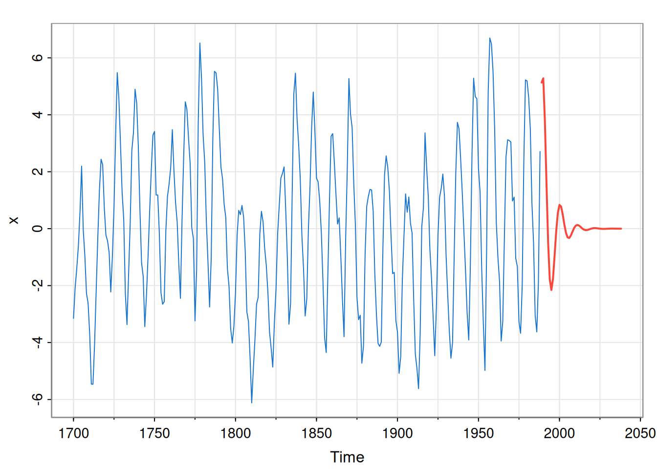
So, the short term forecasts oscillate in line with the recent observations, but the longer term forecasts quickly decay away to the stationary mean of zero as we become increasingly uncertain about the phase of the signal.
4.2.2.2 Forecast variance
Let us now turn attention to the forecast variances. Again, let’s compute them sequentially, starting with the one-step ahead variance. \[\begin{align*} \mathbb{V}\mathrm{ar}[X_{n+1}|\mathbf{X}_{1:n}=\mathbf{x}_{1:n}] &= \mathbb{V}\mathrm{ar}\left[\left.\sum_{j=1}^p \phi_j X_{n+1-j} + \varepsilon_{n+1}\right|\mathbf{X}_{1:n}=\mathbf{x}_{1:n}\right] \\ &= \mathbb{V}\mathrm{ar}\left[\left.\sum_{j=1}^p \phi_j x_{n+1-j} + \varepsilon_{n+1}\right|\mathbf{X}_{1:n}=\mathbf{x}_{1:n}\right] \\ &= \mathbb{V}\mathrm{ar}\left[\left. \varepsilon_{n+1}\right|\mathbf{X}_{1:n}=\mathbf{x}_{1:n}\right] \\ &= \sigma^2. \end{align*}\] Next, let’s consider the 2-step ahead forecast variance, \[\begin{align*} \mathbb{V}\mathrm{ar}[X_{n+2}|\mathbf{X}_{1:n}=\mathbf{x}_{1:n}] &= \mathbb{V}\mathrm{ar}\left[\left.\sum_{j=1}^p \phi_j X_{n+2-j} + \varepsilon_{n+2}\right|\mathbf{X}_{1:n}=\mathbf{x}_{1:n}\right] \\ &= \mathbb{V}\mathrm{ar}\left[\left.\phi_1X_{n+1} + \sum_{j=2}^p \phi_j x_{n+2-j} + \varepsilon_{n+2}\right|\mathbf{X}_{1:n}=\mathbf{x}_{1:n}\right] \\ &= \phi_1^2\mathbb{V}\mathrm{ar}\left[\left.X_{n+1}\right|\mathbf{X}_{1:n}=\mathbf{x}_{1:n}\right] + \sigma^2 \\ &= (1+\phi_1^2 )\sigma^2. \end{align*}\] Beyond this, things start to get a bit more complicated, due to the covariances between observations. Nevertheless, we can continue to slog out the variances using successive substitution. \[\begin{align*} \mathbb{V}\mathrm{ar}[X_{n+3}|\mathbf{X}_{1:n}=\mathbf{x}_{1:n}] &= \mathbb{V}\mathrm{ar}\left[\left.\sum_{j=1}^p \phi_j X_{n+3-j} + \varepsilon_{n+3}\right|\mathbf{X}_{1:n}=\mathbf{x}_{1:n}\right] \\ &= \mathbb{V}\mathrm{ar}\left[\left.\phi_1X_{n+2}+\phi_2X_{n+1}+ \sum_{j=3}^p \phi_j x_{n+3-j} + \varepsilon_{n+3}\right|\mathbf{X}_{1:n}=\mathbf{x}_{1:n}\right] \\ &= \mathbb{V}\mathrm{ar}\left[\left.\phi_1X_{n+2}+\phi_2X_{n+1}\right|\mathbf{X}_{1:n}=\mathbf{x}_{1:n}\right] +\sigma^2 \\ &= \mathbb{V}\mathrm{ar}\left[\left.\phi_1\left(\phi_1X_{n+1}+\sum_{j=2}^p\phi_k x_{n+2-j}+\varepsilon_{n+2}\right)+\phi_2X_{n+1}\right|\mathbf{X}_{1:n}=\mathbf{x}_{1:n}\right] +\sigma^2 \\ &= \mathbb{V}\mathrm{ar}\left[\left. (\phi_1^2+\phi_2)X_{n+1} + \phi_1\varepsilon_{n+2} \right|\mathbf{X}_{1:n}=\mathbf{x}_{1:n}\right] +\sigma^2 \\ &= (\phi_1^2+\phi_2)^2\mathbb{V}\mathrm{ar}\left[\left. X_{n+1} \right|\mathbf{X}_{1:n}=\mathbf{x}_{1:n}\right] +(1+\phi_1^2)\sigma^2 \\ &= \left(1+\phi_1^2+[\phi_1^2+\phi_2]^2\right)\sigma^2 \end{align*}\] It is possible to derive recursions that give the forecast variances, but it is probably not worth it. Note that the case of the AR(1) was dealt with in Chapter 2, where explicit forecast distributions were derived. The initial condition there becomes the final observation, \(x_n\), here. Similarly, we can write an AR(p) as a VAR(1), and use the explicit expressions for the forecast variance for the VAR(1) from Chapter 2 to deduce the forecast variance for the AR(p).
In practice, we just use the arima function to compute forecasts and associated uncertainties.
mod = arima(x, c(2,0,0))
fore = predict(mod, n.ahead=k)
pred = fore$pred
sds = fore$se
tsplot(x, xlim=c(tsp(x)[1], tsp(x)[2]+k),
  ylim=c(-10, 10), col=4)
ftimes = seq(tsp(x)[2]+1, tsp(x)[2]+k, tsp(x)[3])
lines(ftimes, pred, col=2, lwd=2)
lines(ftimes, pred+2*sds, col=2)
lines(ftimes, pred-2*sds, col=2)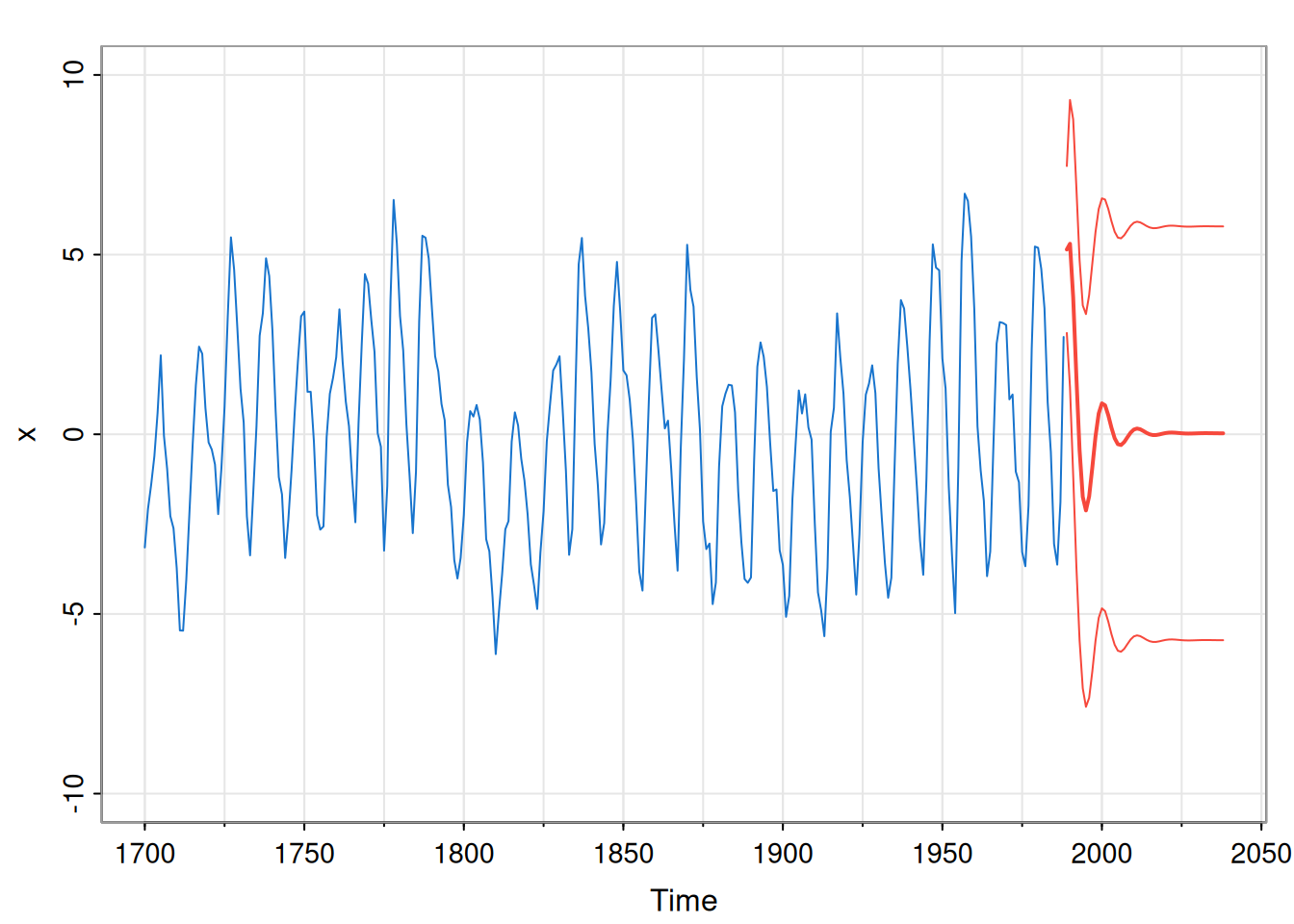
4.2.3 Forecasting an ARMA(p,q)
As usual, the case of an ARMA model is similar to that of an AR model, but a little bit more complicated due to the extra error terms. Recall from our discussion of conditional least squares and conditional likelihood approaches to model fitting, that for long time series, there is a deterministic relationship between \(x_t\) and \(\varepsilon_t\). Just as we can simulate an ARMA model by applying an ARMA filter to white noise, we can also recover the error process by applying an ARMA filter to the time series. In the context of forecasting, this means that if we know the observed values of the time series up to time \(n\), we also know the observed values of the errors up to time \(n\). We will denote these \(\tilde\varepsilon_1,\tilde\varepsilon_2,\ldots,\tilde\varepsilon_n\) in order to emphasise that these are observed and not random. Given this, we can just proceed as before. It is clear that the one-step ahead predictive variance for any ARMA model will be \(\sigma^2\), but variance forecasts further ahead get quite cumbersome quite quickly. The (mean) forecast function, \(\hat{x}_n(k)\), is more straightforward.
For the ARMA model \[ X_t = \sum_{j=1}^p \phi_jX_{t-j} + \sum_{j=1}^q\theta_j\varepsilon_{t-j}+\varepsilon_t, \] we have \[\begin{align*} \hat{x}_n(k) &= \mathbb{E}\left[\left. X_{n+k} \right|\mathbf{X}_{1:n}=\mathbf{x}_{1:n},\pmb{\varepsilon}_{1:n}=\tilde{\pmb{\varepsilon}}_{1:n}\right] \\ &= \mathbb{E}\left[\left. \sum_{j=1}^p \phi_jX_{n+k-j} + \sum_{j=1}^q\theta_j\varepsilon_{n+k-j} + \varepsilon_t \right|\mathbf{X}_{1:n}=\mathbf{x}_{1:n},\pmb{\varepsilon}_{1:n}=\tilde{\pmb{\varepsilon}}_{1:n}\right] \\ &= \sum_{j=1}^p \phi_j\mathbb{E}[X_{n+k-j}|\mathbf{X}_{1:n}=\mathbf{x}_{1:n}] + \sum_{j=1}^q \theta_j\mathbb{E}[\varepsilon_{n+k-j}|\pmb{\varepsilon}_{1:n}=\tilde{\pmb{\varepsilon}}_{1:n}]. \end{align*}\] Now we define \(\hat{x}_n(-t)=x_{n-t}\) for \(t\geq 0\), as before, and also now define \(\tilde\varepsilon_t=0\) for \(t>n\), to get \[ \hat{x}_n(k) = \sum_{j=1}^p \phi_j \hat{x}_n(k-j) + \sum_{j=1}^q \theta_j\tilde{\varepsilon}_{n+k-j}. \tag{4.2}\] So for \(k=1,2,\ldots,q\) we explicitly enumerate \(\hat{x}_n(k)\) using Equation 4.2, and then for \(k>q\) we have the linear recurrence \[ \hat{x}_n(k) = \sum_{j=1}^p \phi_j \hat{x}_n(k-j), \] as for the AR(p).