MATH4341: Spatio-temporal statistics
Term 2: Spatial modelling and analysis
Computer Lab 6: Spectral synthesis and kriging
Load up RStudio via your favourite method. If you can’t use RStudio for some reason, most of what we do in these labs can probably be done using WebR, but the instructions will assume RStudio. You will also want to have the web version of the lecture notes to refer to.
Question 1
If you haven’t already done so, reproduce all of the plots and computations from Chapter 12 and Chapter 13 of the lecture notes by copying and pasting each code block in turn. Make sure you understand what each block is doing and that you can reproduce all of the plots.
Question 2
In the context of geostatistics, the Matérn covariance function is a very useful, flexible class of covariograms determining (weakly) stationary random fields with varying smoothness levels. But where does it come from?
We know from Bochner’s theorem that valid covariograms are the Fourier transforms of spectral density functions that are integrable non-negative even functions. So every even PDF gives rise to a valid covariogram. We would like a flexible class of covariograms of varying levels of smoothness and differentiability. We also know that the tail behaviour of the spectral density function determines the regularity of the associated stationary process. So we are looking for a class of even PDFs with tunable tail behaviour. Do we know of any PDFs like that? Yes, we do! The PDF of Student’s t-distribution is exactly what we want. If you go to the Wikipedia page for the \(t\)-distribution and look down the summary table on the RHS, you will find the PDF, which has exactly the form we want, and the characteristic function (CF) which looks like the Matérn covariogram. The CF is a form of Fourier transform, so we are clearly on the right track. Note that the CF of the \(t\)-distribution was known long before people were looking for interesting spatial covariograms. Now look the the Wikipedia page for the Matérn covariance function. It gives the covariogram with a very slightly different parameterisation to the one that we used, and the spectral density function, which we can see is essentially the PDF of the \(t\)-distribution. Now, we have presented the covariogram using the parameterisation, \[
C(\mathbf{h}) = \frac{\sigma^2}{2^{\nu-1}\Gamma(\nu)}\left(\frac{\Vert\mathbf{h}\Vert}{\phi}\right)^\nu K_v\left(\frac{\Vert\mathbf{h}\Vert}{\phi}\right),
\] which is the parameterisation used by geoR, and so using our parameterisation, the corresponding spectral density function is \[
S(\mathbf{f}) = \frac{\sigma^2 2^d \pi^{\frac{d}{2}}\Gamma(\nu+\frac{d}{2})}{\Gamma(\nu)\phi^{2\nu}}\left[ \frac{1}{\phi^2} + (2\pi\Vert\mathbf{f}\Vert)^2 \right]^{-(\nu+\frac{d}{2})}
\] Note that here we are exceptionally using \(\mathbf{f}\) for frequency, rather than \(\pmb{\nu}\), since \(\nu\) is already being used for the smoothness parameter. Also note that the spectral density depends on the dimension, \(d\), of the space, \(\mathcal{D}\subset\mathbb{R}^d\), that we are working in (typically, \(d=1\) or 2). We can see that the tail behaviour of this spectral density function is \(\Vert \mathbf{f}\Vert^{-(2\nu+d)}\), and so at this point it should be reasonably clear why the process will be \(k\)-times differentiable iqm, for \(k\in\mathbb{N}\), if \(\nu>k\).
We can use the spectral density function for spectral synthesis of Matérn fields on high-resolution grids. A basic function to evaluate the spectral density function is given below.
It’s easy enough to partially apply this function, as required. eg.
S = function(f) Sm(f, 1, 0.1, 0.8, 1)is a function of a single argument, f, corresponding to the frequency.
Task A
Repeat Tasks B and C of Question 2 from Lab 5, but now using spectral synthesis instead of the covariance matrix method. Note that you will need d=1 for 1-d simulation and d=2 for 2-d simulation. Feel free to use simulation functions from Chapter 12. The versions you simulate using spectral synthesis should look qualitatively similar to those you did using the covariance matrix method in Lab 5.
Task B
Using \(\sigma=1\), \(\phi=0.1\), \(\nu=0.8\), and \(d=2\), simulate a 2-d Matérn field on a \(512\times 512\) grid using spectral synthesis. Note that this would be impractical using the naive covariance matrix method (feel free to try, but be sure to save your work, first!). Try to produce a nice image of the sampled field.
Question 3
For this question we will analyse a dataset in the gstat package, which you might not have installed. If not, install it with install.packages("gstat"), as usual.
Use ?jura to find out a little about the data which originates from the Swiss Jura mountains. It is soil sample data, much like the meuse data, and again, we will focus on zinc concentration. The actual data that we are interested in is in the data frame jura.pred.
dim(jura.pred)[1] 259 13head(jura.pred) Xloc Yloc long lat Landuse Rock Cd Co Cr Cu
1 2.386 3.077 6.850413 47.13907 Meadow Sequanian 1.740 9.320 38.32 25.72
2 2.544 1.972 6.852674 47.12918 Pasture Kimmeridgian 1.335 10.000 40.20 24.76
3 2.807 3.347 6.855886 47.14154 Pasture Sequanian 1.610 10.600 47.00 8.88
4 4.308 1.933 6.875799 47.12899 Meadow Kimmeridgian 2.150 11.920 43.52 22.70
5 4.383 1.081 6.876925 47.12136 Meadow Quaternary 1.565 16.320 38.52 34.32
6 3.244 4.519 6.861415 47.15209 Meadow Quaternary 1.145 3.508 40.40 31.28
Ni Pb Zn
1 21.32 77.36 92.56
2 29.72 77.88 73.56
3 21.40 30.80 64.80
4 29.72 56.40 90.00
5 26.20 66.40 88.40
6 22.04 72.40 75.20plot(jura.pred[,1:2], cex=jura.pred$Zn/100, pch=19, col=4,
main="Measurements of zinc concentration")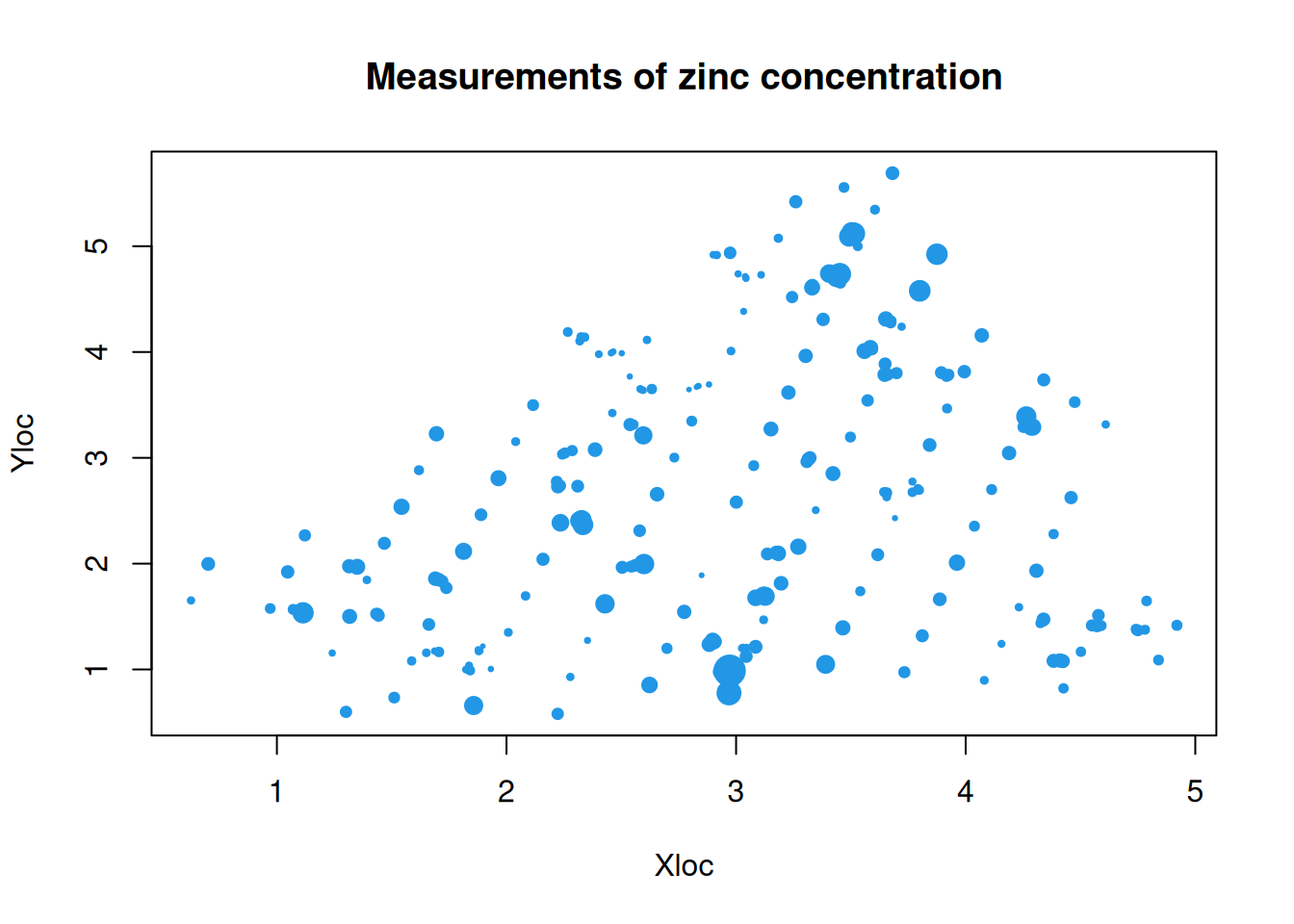
So we can see that we have measured values over a good range of spatial locations, and that there does seem to be variation over space. Since the data frame contains long and lat values, it is easy to turn into an sf object, in case that is required.
jura = st_as_sf(jura.pred, coords=c("long", "lat"), crs=4326)
plot(jura[,"Zn"], pch=19, main="Measurements of zinc concentration")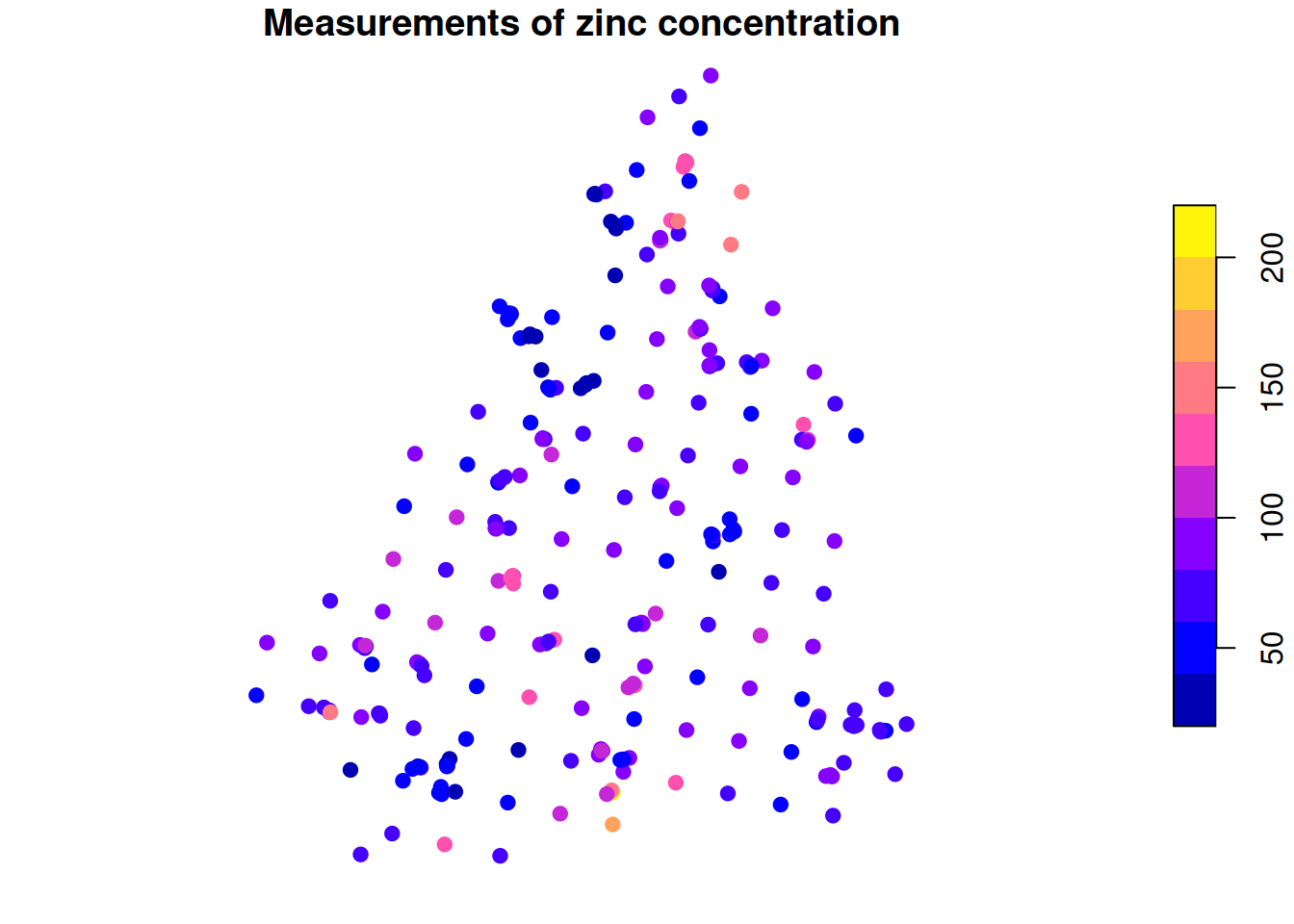
If you installed ggmap and a StadiaMaps API key, then you can look at the data in context. If not, just skip this code block - it is not needed for what follows.
library(ggmap)
jura_bb = st_bbox(jura)
names(jura_bb) = c("left", "bottom", "right", "top") # ggmap-style bb
jura_map = get_map(jura_bb, maptype="stamen_terrain", source="stadia")
ggmap(jura_map)+
    geom_sf(data = jura, mapping=aes(colour=Zn),
            inherit.aes=FALSE) +
    labs(x="Longitude", y="Latitude")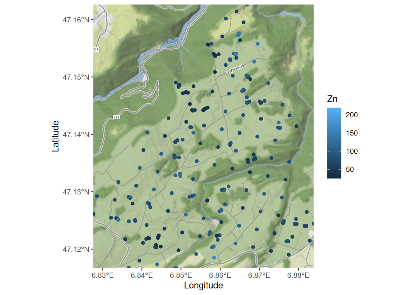
Task C
Your task is to use the geoR package to first fit a (semi-)variogram function to the zinc concentrations and then use kriging to obtain a smooth estimate of zinc concentrations across the study region. You should try fitting variograms using both empirical and maximum likelihood methods and use whatever works best. Once you have the kriging working, you should clip your predictions to just cover the area where the predictive variance isn’t too high. Produce some nice plots.