12 Spectral theory for GPs
12.1 Introduction
In Chapter 5 we saw how we could use Fourier transforms in order to decompose time series models and data into frequency components and how that could give us additional insight into the nature of the process. We would now like to do the same for random fields, and GPs in particular. As usual, we will start with the 1d case and then turn to 2d fields. In Chapter 5 we used three different flavours of Fourier transform: Fourier series, for a continuous function on a finite interval; the discrete time Fourier transform, for a discrete time series model; and the discrete Fourier transform for a finite time series. To represent a continuous random field, we will need another Fourier transform, the continuous Fourier transform, usually referred to simply as the Fourier transform, since it really subsumes all other flavours of Fourier transform as special cases.
For a function \(f:\mathbb{R}\rightarrow\mathbb{C}\), the Fourier transform of \(f\), often denoted \(\hat{f}:\mathbb{R}\rightarrow\mathbb{C}\), is defined by \[ \hat{f}(\nu) = \int_{-\infty}^\infty f(x)e^{-2\pi\mathrm{i}\nu x}\,\mathrm{d}x. \] It can be inverted with the inverse Fourier transform, \[ f(x) = \int_{-\infty}^\infty \hat{f}(\nu)e^{2\pi\mathrm{i}\nu x}\,\mathrm{d}\nu. \] The inverse transform represents the function \(f\) as a continuous mixture of oscillations, with the weight and phase of the oscillation at frequency \(\nu\) being determined by the Fourier transform at that frequency, \(\hat{f}(\nu)\). The inverse transform is almost identical to the inverse transform of the DTFT that we met in Section 5.1.2. However, there we didn’t need any oscillations with frequencies higher than \(1/2\) (the Nyquist frequency), due to only needing to know the function on a grid with a grid spacing of 1. Here, we want to know \(f\) everywhere, so we need all frequencies, and hence we must integrate over the full real line.
That the forward and inverse transforms correctly invert one another follows directly from the key orthogonality property \[ \int_{-\infty}^\infty e^{2\pi\mathrm{i}\nu x}\,\mathrm{d}\nu = \delta(x), \] where, as always, \(\delta(x)\) is Dirac’s delta function. This property can be interpreted as saying that the (inverse) Fourier transform of the constant function, 1, is the delta function. We will see a bit later why it is true. Note that it is clear that both the forward and inverse Fourier transform of the delta function is the constant function, 1.
Using this orthogonality property we can check inversion by considering the inverse transform of the forward transform as \[\begin{align*} \int_\mathbb{R}\mathrm{d}\nu\, \hat{f}(\nu)e^{2\pi\mathrm{i}\nu x} &= \int_\mathbb{R}\mathrm{d}\nu\, \int_\mathbb{R}\mathrm{d}y\,f(y)e^{-2\pi\mathrm{i}\nu y} e^{2\pi\mathrm{i}\nu x} \\ &= \int_\mathbb{R}\mathrm{d}y\, f(y) \int_\mathbb{R}\mathrm{d}\nu\,e^{2\pi\mathrm{i}\nu (x-y)} \\ &= \int_\mathbb{R}\mathrm{d}y\, f(y) \delta(x-y) = f(x). \end{align*}\]
Since these Fourier transforms are now integrals over the whole real line, there are potentially issues of integrability and convergence. The transforms will clearly exist for integrable functions, but the class of functions for which transforms exist can be generalised beyond this (for example, to a constant function, as above). We will largely ignore such technicalities.
It is possible to analytically compute the Fourier transform of many functions, but this often requires some knowledge of complex analysis. Fortunately, the transforms for many functions can be found in Fourier transform tables. Using these, together with the fact that the Fourier transform is linear, allows the computation of Fourier transforms for many functions of interest.
12.2 Spectral representation
We would like to use Fourier transforms to understand random fields. If a random field, \(Z(s)\), has a Fourier transform, \(\hat{Z}(\nu)\), then this is also a random field, and vice versa. So, as in Chapter 5, we will consider the random field that is induced by a Fourier transform that is a weighted white noise process, \(\hat{Z}(\nu)=\sigma(\nu)\eta(\nu)\), where \(\sigma(\cdot)\) is a deterministic weighting function that we are free to specify, and \(\eta(\cdot)\) is a white noise process with covariogram equal to Dirac’s delta. We therefore represent \(Z(s)\) as \[ Z(s) = \int_\mathbb{R} \sigma(\nu)e^{2\pi\mathrm{i}\nu s}\eta(\nu)\,\mathrm{d}\nu, \] so that \(Z(s)\) is a random continuous mixture of frequency components. Again, it may be preferable to write this as an integral wrt a Wiener process as \[ Z(s) = \int_\mathbb{R} \sigma(\nu)e^{2\pi\mathrm{i}\nu s}\mathrm{d}W(\nu), \] which arguably makes it easier to see that \(Z(s)\) will be a GP. Taking expectations gives \(\mathbb{E}[Z(s)]=0,\forall s\in\mathbb{R}\), so \(Z(s)\) is a mean zero GP. We can now compute its covariance function \[\begin{align*} C(s+h, s) &= \mathbb{C}\mathrm{ov}[Z(s+h),Z(s)] \\ &= \mathbb{E}\left[Z(s+h)\overline{Z(s)}\right] \\ &= \int_\mathbb{R} |\sigma(\nu)|^2e^{2\pi\mathrm{i}h\nu}\,\mathrm{d}\nu, \end{align*}\] following exactly the same derivation as in Section 5.2. Since this is independent of \(s\), we conclude that the process is stationary, and defining the spectral density, \(S(\nu) = |\sigma(\nu)|^2\) (so clearly real and non-negative), we can write the covariogram as \[ C(h) = \int_\mathbb{R} S(\nu)e^{2\pi\mathrm{i}h\nu}\,\mathrm{d}\nu. \] Consequently, \(C(\cdot)\) is the inverse Fourier transform of \(S(\cdot)\), and so the spectral density is the Fourier transform of the covariogram, \[ S(\nu) = \int_\mathbb{R}C(h)e^{-2\pi\mathrm{i}h\nu}\,\mathrm{d}h. \] The covariogram and spectral density form a Fourier transform pair.
We know that for a (real) stationary GP, the covariagram is real and even, so (if we prefer) we can write the spectral density as \[ S(\nu) = 2\int_0^\infty C(h)\cos(2\pi h\nu)\,\mathrm{d}h, \] and so \(S(\cdot)\) is also even, in which case we can also write \[ C(h) = 2\int_0^\infty S(\nu)\cos(2\pi h\nu)\,\mathrm{d}\nu. \] The stationary variance of the induced process is \[ C(0) = \int_\mathbb{R} S(\nu)\,\mathrm{d}\nu, \] and so to obtain a weakly stationary GP (with finite variance), \(S(\cdot)\) must be integrable. Since any non-negative even integrable function \(S(\cdot)\) induces a weakly stationary GP, the induced covariogram must be valid (positive definite). This gives us a recipe for constructing valid covariograms: pick any non-negative even integrable function and compute its inverse Fourier transform to get a valid covariogram. As statisticians, we know lots of non-negative integrable functions - probability density functions (PDFs). So, just start with any (possibly scaled) even PDF and compute its inverse Fourier transform. Conversely, we also have a mechanism for checking whether a given covariogram is valid: compute its Fourier transform and check that it is real, non-negative, even, and integrable.
As usual, we have glossed over many technicalities and conditions. Precise results formalising our analysis include the Wiener–Khinchin theorem and Bochner’s theorem. The Karhunen–Loève theorem is also somewhat relevant. That the spectral density and covariogram form a Fourier transform pair is often referred to by statisticians as Bochner’s theorem.
12.3 Examples
12.3.1 Squared-exponential covariogram
Let us start by considering the function \(f(x) = e^{-\alpha x^2}\). It is not too difficult to compute the Fourier transform of this function directly, but we can also look it up in tables to find \[ \hat{f}(\nu) = \sqrt{\frac{\pi}{\alpha}} \exp\{-\pi^2\nu^2/\alpha\}. \] So the transform of a squared-exponential function is squared-exponential. Furthermore, using the Gaussian integral, or otherwise, we see that the transform is a correctly normalised Gaussian PDF (that is, it integrates to 1). However, the length scales are reciprocals. As \(\alpha\rightarrow 0\), \(f(x)\) tends to the constant function, 1, whereas \(\hat{f}(\nu)\) tends to the delta function, \(\delta(\nu)\). This is a good way to understand the key orthogonality property we needed to establish invertibility.
If we now think about a squared-exponential covariogram parameterised the usual way \[ C(h) = \sigma^2e^{-(h/\phi)^2}, \] we can Fourier transform it to get \[ S(\nu) = \sigma^2\phi\sqrt{\pi}\,e^{-(\pi\phi\nu)^2}. \] When the length scale, \(\phi\), is large, the covariogram is broad, corresponding to variations over large distances. In this case, the spectrum is narrow and sharply peaked around zero, since the process is dominated by low frequency oscillations. Conversely, when \(\phi\) is small, the covariogram is concentrated near zero, due to correlations persisting over only short length scales. But the spectrum is broad, reflecting the fact that the process is composed of oscillations over a wide range of frequencies.
We have already noted that the delta function transforms to the constant function. Consequently, white noise has a completely flat spectrum, corresponding to the fact that the process is made up from oscillations at all frequencies equally.
12.3.2 Exponential covariogram (OU process)
We start by considering the function \(f(x) = e^{-a|x|}\). From tables, we find that \[ \hat{f}(\nu) = \frac{2a}{a^2+4\pi^2\nu^2}. \] So, the spectrum is in the form of a Cauchy distribution, and careful inspection reveals that this is, again, correctly normalised (and again, the \(a\rightarrow 0\) limit corresponds to the constant function transforming to the delta function).
We have seen two different commonly encountered ways of parameterising the exponential covariogram. In the context of spatial statistics, it is most common to write it as \[ C(h) = \sigma^2e^{-|h|/\phi}. \] We can Fourier transform this to obtain \[ S(\nu) = \frac{2\sigma^2\phi}{1+(2\pi\phi\nu)^2}. \] The spectrum has long tails relative to a squared-exponential, reflecting the fact that there is always a mixture across a broad frequency range, irrespective of the length scale (this contributes to the roughness of sample paths). Nevertheless, the reciprocal nature of the length scales is the same as for the squared-exponential covariogram. When the covariogram length scale is large, the spectrum is concentrated close to zero (low frequencies), and vice versa.
12.4 Spectral synthesis and the FFT
We can use the spectral representation to simulate realisations of stationary GPs. Given a spectrum, \(S(\nu)\) we have the representation \[ Z(s) = \int_\mathbb{R} \sqrt{S(\nu)} e^{2\pi\mathrm{i}\nu s}\eta(\nu)\,\mathrm{d}\nu, \] and so in principle we just need to inverse Fourier transform a realisation of the random function \(\sqrt{S(\nu)}\eta(\nu)\). This isn’t something we can do exactly on a computer, but is something we can do approximately, as accurately as we want, on a grid as fine as we want, by approximating the integral as a Riemann sum. There are many ways that we could do this, but if we do it in just the right way, we can express the sum in the form of an inverse DFT, which will then allow us to use the (inverse) FFT to do the computation. Before diving into the details, it is worth dwelling on why this is worth bothering with. After all, we already know how to simulate realisations of GPs, using the covariance matrix approach. But as previously mentioned, to simulate on \(n\) grid points, that approach is \(\mathcal{O}(n^2)\) in storage and \(\mathcal{O}(n^3)\) in computation, making it infeasible for large dense grids in 2 and 3 dimensions. The approach we develop here is \(\mathcal{O}(n)\) in storage. Using a naive DFT implementation would be \(\mathcal{O}(n^2)\) in computation, which is already much better than the covariance matrix approach. But using the FFT will reduce the computational cost to \(\mathcal{O}(n\log n)\), making it very practical even for large dense grids in 2 and 3 dimensions.
First we need to discretise space. We choose a required number of grid points, \(n\), and the grid spacing \(\Delta s\). Then for \(j=0,1,\ldots,n-1\) we define \(Z_j = Z(j\Delta s)\) and re-write our representation as the Itô integral \[ Z_j = \int_\mathbb{R} \sqrt{S(\nu)}e^{2\pi\mathrm{i}\nu j\Delta s}\,\mathrm{d}W(\nu). \] We now consider approximating the integral as a Riemann sum by discretising the frequency range. To get the approximation in the form of a DFT we need to choose \(n\) frequency levels. For now we will consider an arbitrary frequency step size \(\Delta\nu\). Our Riemann sum takes the form \[ Z_j \simeq \sum_{k=-n/2}^{n/2-1} \sqrt{S(k\Delta\nu)}\,e^{2\pi\mathrm{i}k\Delta\nu j\Delta s}\sqrt{\Delta\nu}W_k, \] where the \(W_k\) are iid mean zero Gaussian random variables with variance one. The factor of \(\sqrt{\Delta \nu}\) comes from the fact that the integrated noise over an interval of width \(\Delta\nu\) will have variance \(\Delta\nu\), and we choose to construct it from a quantity of variance one and then multiply it by \(\sqrt{\Delta\nu}\). We then notice that by choosing \(\Delta\nu = 1/(n\Delta s)\) we get \[ Z_j \simeq \sum_{k=-n/2}^{n/2-1} \sqrt{\frac{S(k/[n\Delta s])}{n\Delta s}}W_k e^{2\pi\mathrm{i}k j/n}, \] which is now of exactly the right form for a DFT (modulo some indexing issues that we will fix presently). Something that we have so far glossed over now becomes important: the white noise in the spectral representation has to be complex, in order to have random phase shifts of the oscillations at each frequency, as well as random amplitudes. This means that the \(W_k\) have to be standard complex normal random quantities, \(\mathcal{CN}(0,1)\). We can construct these from two standard normal random quantities \(U,V\sim\mathcal{N}(0,1)\) as \(W_k = (U + \mathrm{i}V)/\sqrt{2}\). Note the factor of \(\sqrt{2}\), which ensures that the variance of \(W_k\) is 1. We can now define \[ X_k = \sqrt{\frac{S(k/[n\Delta s])}{n\Delta s}}W_k, \] to get \[ Z_j \simeq \sum_{k=-n/2}^{n/2-1} X_k\, e^{2\pi\mathrm{i}k j/n} \] Since we ultimately want a real-valued process, \(Z_j\), we actually simulate the \(X_k\) for \(k=0,1,\ldots,n/2-1\), and then set \(X_{-k}=\overline{X}_k\). Now we fix the indexing, and write \[ Z_j \simeq \sum_{k=0}^{n-1} X_k\, e^{2\pi\mathrm{i}k j/n}, \] where now we set \(X_{n-k}=\overline{X}_k\), and we must also ensure that \(X_0\) and \(X_{n/2}\) are both real. Finally, since the inverse DFT conventionally includes the factor of \(n\), we can define \[ Y_k = n X_k = \sqrt{\frac{n S(k/[n\Delta s])}{\Delta s}}W_k, \] to get \[ Z_j \simeq \frac{1}{n}\sum_{k=0}^{n-1} Y_k\, e^{2\pi\mathrm{i}k j/n}, \] which is now precisely the inverse DFT of the \(Y_k\). So, to generate our stationary GP, we iid simulate the \(Y_k\), which is easy, then apply the inverse DFT to get our process realisation. Although it was a little bit of work to figure out the procedure, it is very straightforward to implement and use in practice.
First we need our function for inverting the DFT, and a function for simulating (standard) complex normals.
We can check that this seems to work and gives us random quantities with a variance of one as follows.
[1]  0.96941401+1.6440646i -0.39930191+0.3706103i  0.25677056+0.6864122i
[4] 0.44750144+0.2665604i 0.28586087-0.7042313i -0.07504136-0.4224842i[1] 0.9880415Now we can create a function to take in a spectral function and follow the recipe we outlined above to give us an approximate GP realisation on our required grid.
rgp = function(n, S_fun, upper=1, ...) {
    delta_s = upper/n # simulate on [0, upper)
    k = 0:(n-1)
    s = S_fun(k/(n*delta_s), ...)
    if (is.na(s[1]))
        s[1] = 0 # fix if spectrum blows up at 0
    Y = sqrt(s*n/delta_s)*rcnorm(n)
    Y[1] = Re(Y[1]) # real coef at freq 0
    Y[n/2+1] = Re(Y[n/2+1]) # real coef at freq 1/2
    Y[(n/2 + 2):n] = rev(Conj(Y[2:(n/2)])) # set neg freqs to conj
    ts(Re(ifft(Y)), start=0, deltat=delta_s)
}
We can test this out with a squared-exponential covariance function as follows.
S_se = function(nu, phi=0.1)
    phi*sqrt(pi)*exp(-(pi*phi*nu)^2)

Z = rgp(n, S_se)
plot(Z, col=4, lwd=2, main="Squared-exponential covariogram")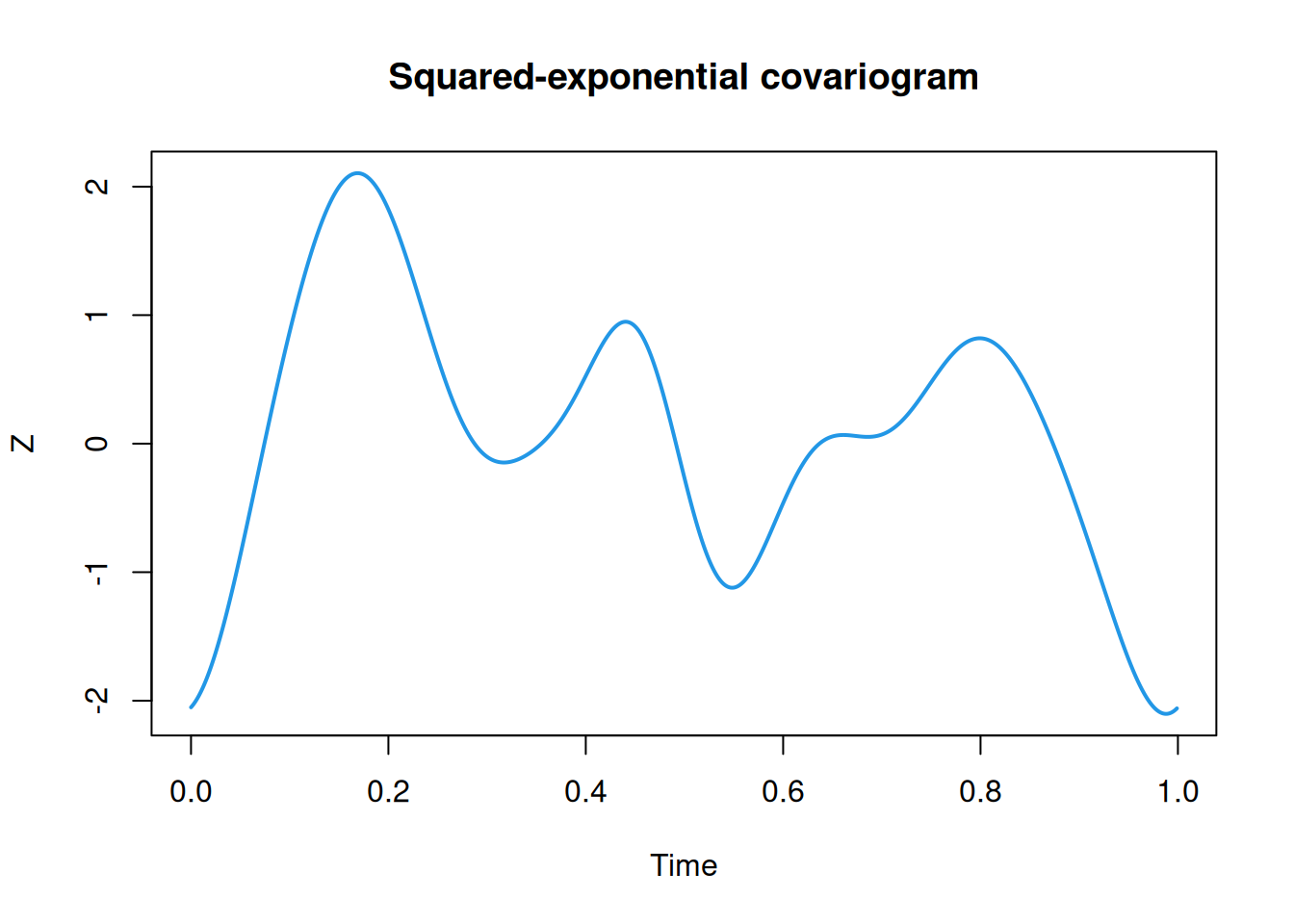
We can contrast this with an exponential covariogram (OU process).
S_exp = function(nu, phi=0.2)
    2*phi/(1 + (2*pi*phi*nu)^2)

Z = rgp(n, S_exp)
plot(Z, col=4, lwd=2, main="OU process")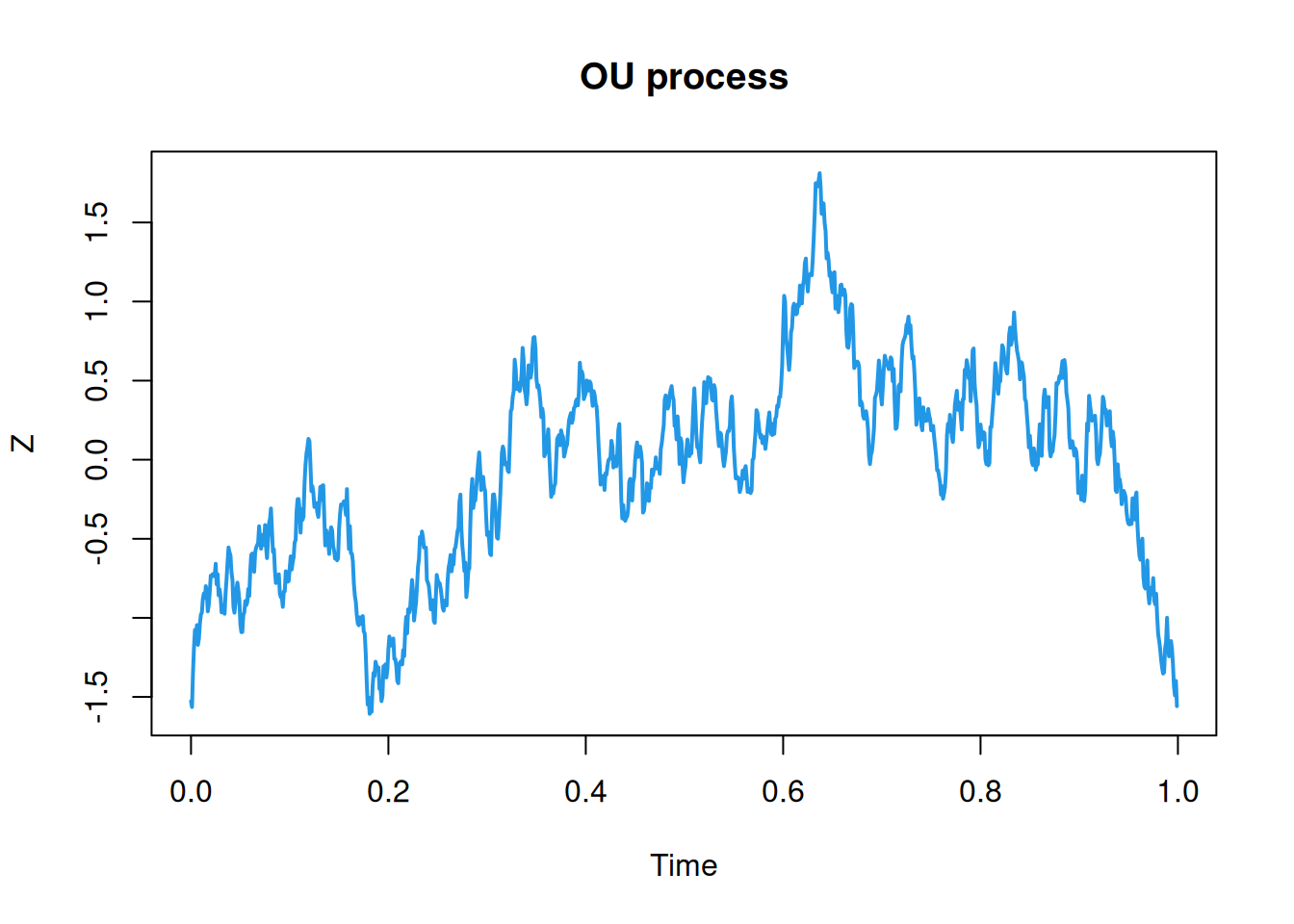
We can hopefully see that these are at least qualitatively similar to the realisations obtained from the exact covariance function method outlined in the previous chapter. But these realisations are obtained at a fraction of the computational cost.
12.4.1 Synthesising intrinsically stationary processes
Our approach to spectral synthesis always gives rise to stationary GPs, so can’t be applied directly to non-stationary intrinsically stationary processes. However, the approach can often be easily adapted using the fact that although the process itself is not stationary, its increments are.
We will begin with the almost trivial example of Wiener process to get the idea, and then look at the more interesting case of fBM. Again, we must choose a grid spacing, \(\Delta s\), and the required number of grid points, \(n\). We can then define the increment process \[ Y_{\Delta s}(s) = W(s+\Delta s) - W(s) \sim \mathcal{N}(0,\Delta s). \] So in this particularly special (Markovian) case, the increments are not only stationary, but iid (a nugget process). So we don’t need any spectral theory to simulate them. Put \(Y_j = Y_{\Delta s}(j\Delta s),\ j=0,1,\ldots,n-1\), and \(W_j=W(j\Delta s)\), then after simulating the iid \(Y_j\sim \mathcal{N}(0,\Delta s)\) we can form the cumulative sums \[ W_j = \sum_{k=0}^{j-1} Y_k, \quad j=1,2,\ldots,n-1, \] to get our non-stationary Wiener process (with \(W_0=0\)).
delta_s = 1/n
Y = rnorm(n, 0, sqrt(delta_s))
W = ts(cumsum(Y), start=0, deltat=delta_s)
plot(W, col=4, lwd=2, main="Wiener process")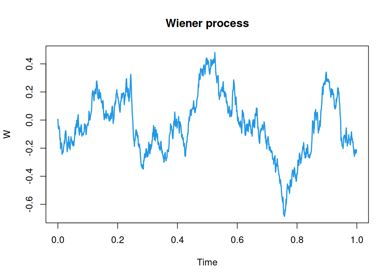
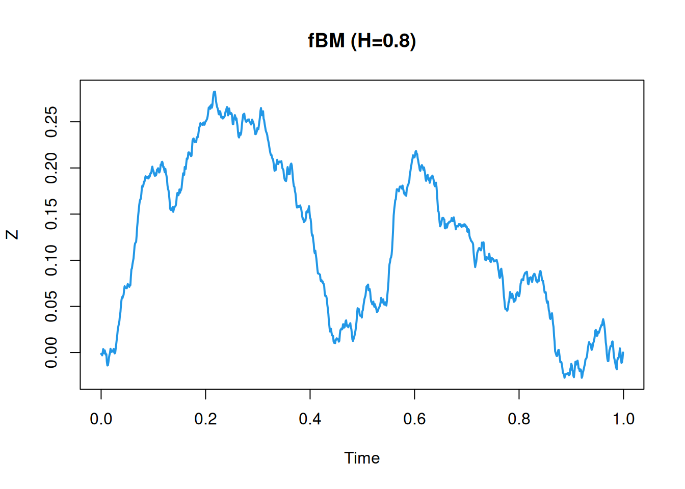
Now we have established the basic idea, we can think about the more interesting case of fBM. This is a process, \(Z(s)\), with semi-variogram \(\gamma(s)=|s|^{2H}/2\) (for some given fixed Hurst exponent, \(H\in(0,1)\)). We again choose a grid spacing, \(\Delta s\), and form the increment process \[ Y_{\Delta s}(s) = Z(s+\Delta s) - Z(s). \] We know that this is a stationary process with stationary variance \(|\Delta s|^{2H}\), but in general this is not a nugget process. It is sometimes referred to as fractional Gaussian noise (fGn). To proceed, we compute its covariogram directly as \[\begin{align*} C_{\Delta s}(s, s+h) &= \mathbb{C}\mathrm{ov}[Y_{\Delta s}(s), Y_{\Delta s}(s+h) \\ &= \mathbb{C}\mathrm{ov}[Z(s+\Delta s)-Z(s), Z(s+h+\Delta s)-Z(s+h)] \\ &= C(s+\Delta s, s+h+\Delta s) - C(s+\Delta s,s+h) \\ &\qquad\qquad\qquad- C(s, s+h+\Delta s) + C(s, s+h) \\ &= \gamma(h+\Delta s) + \gamma(h-\Delta s) - 2\gamma(h). \end{align*}\] This is independent of \(s\), as we would expect, so the covariogram is \[\begin{align*} C_{\Delta s}(h) &= \gamma(h+\Delta s) + \gamma(h-\Delta s) - 2\gamma(h)\\ &= \frac{1}{2}\left\{ |h+\Delta s|^{2H} + |h-\Delta s|^{2H} - 2|h|^{2H} \right\}. \end{align*}\] From this we can confirm that \(C_{\Delta s}(0)=|\Delta s|^{2H}\), as we would hope. We can also compute the covariance between adjacent increments, \(C_{\Delta s}(\Delta s) = (2^{2H-1}-1)|\Delta s|^{2H}\). We confirm that this is 0 for \(H=1/2\), but greater than zero for \(H\in(1/2,1)\) (positively correlated increments) and less than zero for \(H\in(0,1/2)\) (negatively correlated increments). To use spectral synthesis we must compute the spectral density associated with this covariogram using the Fourier transform. From tables, the key results we need are that the transform of \(|x|^\alpha\) is \(-2\sin(\pi\alpha/2)\Gamma(\alpha+1)/|2\pi\nu|^{\alpha+1}\) and that the transform of \(f(x-a)\) is \(e^{-2\pi\mathrm{i}\nu a}\hat{f}(\nu)\). We can then compute the spectral density as \[\begin{align*} S(\nu) &= \frac{\sin(H\pi)\Gamma(2H+1)}{|2\pi\nu|^{2H+1}}\left\{2 - e^{2\pi\mathrm{i}\nu\Delta s} - e^{-2\pi\mathrm{i}\nu\Delta s}\right\} \\ &= \frac{2\sin(H\pi)\Gamma(2H+1)}{|2\pi\nu|^{2H+1}}\left\{1 - \cos(2\pi\nu\Delta s)\right\}. \end{align*}\] We can use this spectral density to synthesise the increment process and then sum it to get a realisation of fBM.
12.5 2d Fourier transforms
To understand the spectral characteristics of 2d random fields, we must first understand 2d Fourier transforms. For a function \(f:\mathbb{R}^2\rightarrow\mathbb{C}\), which we might write as \(f(\mathbf{s})\) or \(f(x, y)\), where \(\mathbf{s}=(x,y)^\top\), we compute the Fourier transform by first (1d) Fourier transforming the first (\(x\)) coordinate holding \(y\) fixed to get a function of \(\nu_x\) and \(y\). We then transform the \(y\) coordinate holding \(\nu_x\) fixed to get a function of \(\nu_x\) and \(\nu_y\), \(\hat{f}(\nu_x, \nu_y)\). In fact, as will become clear, the order in which we transform the coordinates doesn’t actually matter. The result is the same.
Starting from \(f(x,y)\), first transform \(x\): \[ \tilde{f}(\nu_x, y) = \int_\mathbb{R} \mathrm{d}x\, f(x, y)e^{-2\pi\mathrm{i}\nu_x x}. \] Now take this function and transform the \(y\) coordinate: \[\begin{align*} \hat{f}(\nu_x,\nu_y) &= \int_\mathbb{R} \mathrm{d}y\, \tilde{f}(\nu_x, y) e^{-2\pi\mathrm{i}\nu_y y} \\ &= \int_\mathbb{R} \mathrm{d}y\, \int_\mathbb{R} \mathrm{d}x\, f(x, y)e^{-2\pi\mathrm{i}\nu_x x} e^{-2\pi\mathrm{i}\nu_y y} \\ &= \int_\mathbb{R} \mathrm{d}y\, \int_\mathbb{R} \mathrm{d}x\, f(x, y) e^{-2\pi\mathrm{i}(\nu_x x + \nu_y y)}. \end{align*}\] It should now be clear that since we can switch the order of integration, the order in which we transform the coordinates doesn’t matter. Writing \(\hat{f}(\pmb{\nu})=\hat{f}(\nu_x,\nu_y)\), we can write the transform more neatly as \[ \hat{f}(\pmb{\nu}) = \int\!\!\!\int_{\mathbb{R}^2} f(\mathbf{s})e^{-2\pi\mathrm{i}\pmb{\nu}^\top\mathbf{s}}\,\mathrm{d}\mathbf{s}, \] which also has obvious higher-dimensional generalisations. It inverts with \[ f(\mathbf{s}) = \int\!\!\!\int_{\mathbb{R}^2} \hat{f}(\pmb{\nu})e^{2\pi\mathrm{i}\pmb{\nu}^\top\mathbf{s}}\,\mathrm{d}\pmb{\nu}. \]
12.5.1 Spectral representation and Bochner’s theorem
We can now think about spectral representation of 2d random fields. If a 2d random field, \(Z(\mathbf{s})\), has a Fourier transform, \(\hat{Z}(\pmb{\nu})\), then this will also be a random field, and vice versa. So again we consider the random field induced by a weighted (spatial) white noise process. That is, we put \(\hat{Z}(\pmb{\nu}) = \sigma(\pmb{\nu})\eta(\pmb{\nu})\), where \(\sigma(\cdot)\) is a deterministic field that we are free to choose, and \(\eta(\cdot)\) is a spatial white noise process with covariogram \(\delta(\pmb{\nu}) = \delta(\nu_x)\delta(\nu_y)\). Similar computations to the 1d case show that the induced field is mean zero and stationary with covariogram \[ C(\mathbf{h}) = \int\!\!\!\int_{\mathbb{R}^2} S(\pmb{\nu})e^{2\pi\mathrm{i}\pmb{\nu}^\top\mathbf{h}}\,\mathrm{d}\pmb{\nu} = \int\!\!\!\int_{\mathbb{R}^2} S(\pmb{\nu})\cos(2\pi\pmb{\nu}^\top\mathbf{h})\,\mathrm{d}\pmb{\nu}, \] where \(S(\pmb{\nu})=|\sigma(\pmb{\nu})|^2\). This is a 2d inverse Fourier transform and so the corresponding forward transform is \[ S(\pmb{\nu}) = \int\!\!\!\int_{\mathbb{R}^2} C(\mathbf{h})e^{-2\pi\mathrm{i}\pmb{\nu}^\top\mathbf{h}}\,\mathrm{d}\mathbf{h} = \int\!\!\!\int_{\mathbb{R}^2} C(\mathbf{h})\cos(2\pi\pmb{\nu}^\top\mathbf{h})\,\mathrm{d}\mathbf{h}. \]
12.5.2 Examples
12.5.2.1 Squared-exponential covariogram
In principle we can compute 2d Fourier transforms using our knowledge of 1d Fourier transforms, but in practice, we can often either compute them directly or look them up in \(n\)-d tables. From tables we find that \(\exp\{-\frac{1}{2}\mathbf{x}^\top\mathsf{\Sigma}^{-1}\mathbf{x}\}\) transforms to \(2\pi|\mathsf{\Sigma}|^{1/2}\exp\{-2\pi^2\pmb{\nu}^\top\mathsf{\Sigma}\pmb{\nu}\}\) (in the 2d case). So by choosing \(\mathsf{\Sigma}=\frac{1}{2}\phi^2\mathbb{I}\), we find that the covariogram \[ C(\mathbf{h}) = \sigma^2 e^{-\Vert\mathbf{h}\Vert^2/\phi^2} \] transforms to \[ S(\pmb{\nu}) = \sigma^2\phi^2\pi e^{-(\pi\phi\Vert\pmb{\nu}\Vert)^2} . \]
12.5.2.2 Exponential covariogram
From tables, we find that \(\exp\{-2\pi\alpha\Vert \mathbf{x}\Vert\}\) transforms to \[ \frac{\alpha}{2\pi(\alpha^2+\Vert\pmb{\nu}\Vert^2)^\frac{3}{2}}, \] in the 2d case. So, choosing \(\alpha=1/(2\pi\phi)\), the covariogram \[ C(\mathbf{h}) = \sigma^2 e^{-\Vert\mathbf{h}\Vert/\phi} \] transforms to \[ S(\pmb{\nu}) = \frac{\sigma^2}{4\pi^2\phi\left(\frac{1}{4\pi^2\phi^2} + \Vert\pmb{\nu}\Vert^2\right)^\frac{3}{2}}. \]
12.5.3 2d spectral synthesis
Spectral synthesis for 2d stationary GPs proceeds almost identically to the 1d case. A 2d spectral density function must be used, and the approximation is done using a 2d DFT. The 2d DFT of a matrix is obtained by first applying the (1d) DFT to each column of the matrix, and then applying the DFT to each row of the resulting matrix (or vice versa, since again the order doesn’t matter). It inverts in the obvious way. The fft function in R will automatically compute the 2d DFT if given a matrix as input.
For spectral synthesis, a matrix representing the 2d DFT of the process is constructed, and then inverted using the 2d FFT to get a realisation of the 2d process. The most fiddly part of the procedure is ensuring that all of the necessary 2d conjugate symmetries are respected, in order to give rise to a real-valued process. The details of exactly how to do this are not examinable for this course, but a function to implement the procedure is given below.
rgp2d = function(n, S_fun, upper=1, ...) {
    delta_s = upper/n
    d = matrix(0,n,n)
    d = sqrt((row(d)-1)^2 + (col(d)-1)^2)
    s = S_fun(d/(n*delta_s), ...)
    if (is.na(s[1,1]))
        s[1,1] = 0
    y = n*sqrt(s*n/delta_s)*matrix(rcnorm(n*n),n,n)
    y[2:(n/2), (n/2 + 2):n] = y[2:(n/2), (n/2):2]
    y[(n/2 + 2):n, 2:(n/2)] = Conj(y[(n/2):2, 2:(n/2)])
    y[1:(n/2), 1:(n/2)] = n*sqrt(s[1:(n/2), 1:(n/2)]*n/delta_s) *
        matrix(rcnorm(n*n/4), n/2, n/2)
    y[(n/2 + 2):n, (n/2 + 2):n] = Conj(y[(n/2):2, (n/2):2])
    y[1, (n/2+2):n] = Conj(y[1, (n/2):2])
    y[n/2 + 1, (n/2+2):n] = Conj(y[n/2 + 1, (n/2):2])
    y[(n/2+2):n, 1] = Conj(y[(n/2):2, 1])
    y[(n/2+2):n, n/2 + 1] = Conj(y[(n/2):2, n/2 + 1])
    y[1, 1] = Re(y[1, 1])
    y[n/2 + 1, 1] = Re(y[n/2 + 1, 1])
    y[1, n/2 + 1] = Re(y[1, n/2 + 1])
    y[n/2 + 1, n/2 + 1] = Re(y[n/2 + 1, n/2 + 1])
    Re(ifft(y))
}
We can test this for a 2d (isotropic) squared-exponential spectrum.
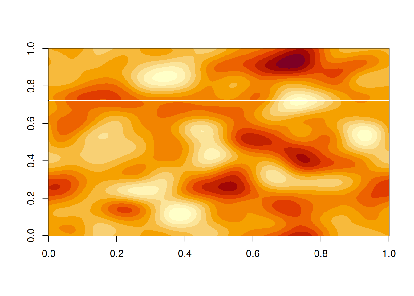

Alternatively, we can use the spectrum for a 2d exponential covariogram.
S_exp2d = function(nu, phi=0.1)
    1/(4*pi*pi*phi*(1/(2*pi*phi)^2 + nu^2)^1.5)

z = rgp2d(n, S_exp2d, phi=0.15)
image(z)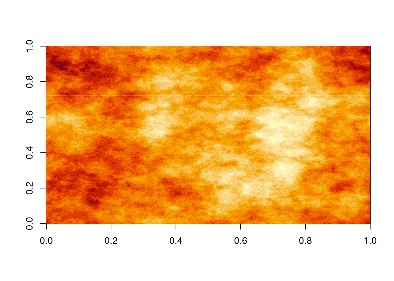
image(z, col=topo.colors(100))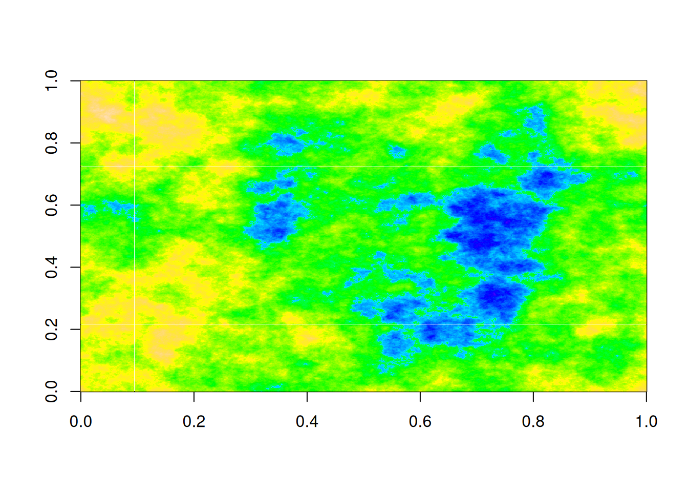
Note that these images are \(1,000\times 1,000\) (one megapixel). It would be completely impractical to simulate 2d fields at this resolution using the naive covariance matrix method, since it would require the construction and decomposition of a \(1,000,000\times 1,000,000\) matrix. Such a matrix contains \(10^{12}\) elements, so even just storing it would take more than 7 terabytes (in double precision, which would almost certainly be required).