Kriging is concerned with using measurements of a latent field at a number of sites in order to make predictions for the value of the field at other (nearby) sites. It is named after D. G. Krige, who devised it for mining applications, though much of the theory was developed later by G. Matheron. Some of the terminology around kriging, and spatial statistics more generally, reflects some of the early mining applications (such as “nugget”).
13.2 Simple Kriging
We begin by considering the simplest form of kriging, where both the mean and covariance function of the latent field are known. This is a very similar setup to the problem of Gaussian process regression considered in Section 11.6, but here we do not make any distributional assumptions, and instead look to consider a linear predictor for the field at an unknown location of interest, and choose a form for that predictor that is optimal in some appropriate sense. We will use similar notation to Section 11.6, and consider \(z_i=z(\mathbf{s}_i)\) to be the measured value of \(Z_i=Z(\mathbf{s}_i),\ i=1,\ldots,n\), and \(Y=Z(\mathbf{s}^\star)\) to be an unobserved value at a particular site of interest, \(\mathbf{s}^\star\). We will use the notation \(\mathbb{E}[Y]=\mu_U\), \(\mathbb{E}[\mathbf{Z}]=\pmb{\mu}_O\), \(\mathbb{V}\mathrm{ar}[Y]=\sigma^2_U\), \(\mathbb{C}\mathrm{ov}[\mathbf{Z}, Y]=\pmb{\sigma}_{OU}\), and \(\mathbb{V}\mathrm{ar}[\mathbf{Z}]=\mathsf{\Sigma}_O+\sigma^2\mathbb{I}\) (that is, we allow a nugget variance in the observation process). We look to predict \(Y\) using a linear predictor of the form \[
\hat{Y} = \alpha + \pmb{\beta}^\top\mathbf{Z}
\] for \(\alpha\) and \(\pmb{\beta}\) minimising the expected quadratic loss function \[
\mathcal{L}(\alpha, \pmb{\beta}) = \mathbb{E}\left[\left(\hat{Y}-Y\right)^2\right].
\] Such an estimator is sometimes known as the best linear unbiased predictor (BLUP). Expanding the loss function we get \[\begin{align*}
\mathcal{L}(\alpha, \pmb{\beta})
&= \mathbb{E}\left[\left(\alpha + \pmb{\beta}^\top\mathbf{Z} - Y\right)^2\right] \\
&= \mathbb{E}\left[\alpha + \pmb{\beta}^\top\mathbf{Z} - Y\right]^2 + \mathbb{V}\mathrm{ar}\left[\alpha + \pmb{\beta}^\top\mathbf{Z} - Y\right] \\
&= \alpha^2 + (\pmb{\beta}^\top\pmb{\mu}_O)^2 + \mu_U^2 + 2\alpha\pmb{\beta}^\top\pmb{\mu}_O - 2\alpha\mu_U - 2\mu_U\pmb{\beta}^\top\pmb{\mu}_O + \\
& \qquad\qquad \pmb{\beta}^\top(\mathsf{\Sigma}_O + \sigma^2\mathbb{I})\pmb{\beta} + \sigma^2_U - 2\pmb{\beta}^\top\pmb{\sigma}_{OU}
\end{align*}\] after some algebra. Differentiating wrt \(\alpha\) and equating to zero gives \[
\alpha = \mu_U - \pmb{\beta}^\top\pmb{\mu}_O.
\] Differentiating wrt \(\pmb{\beta}\), subbing in for \(\alpha\), and equating to zero gives \[
\pmb{\beta} = (\mathsf{\Sigma}_O + \sigma^2\mathbb{I})^{-1}\pmb{\sigma}_{OU}.
\] Consequently, our BLUP takes the form \[
\hat{Y} = \mu_U + \pmb{\sigma}_{OU}^\top(\mathsf{\Sigma}_O + \sigma^2\mathbb{I})^{-1}(\mathbf{Z}-\pmb{\mu}_O).
\] We can evaluate the predictive uncertainty associated with this BLUP as \[\begin{align*}
\mathbb{V}\mathrm{ar}[\hat{Y}-Y]
&= \mathbb{V}\mathrm{ar}[\mu_U + \pmb{\sigma}_{OU}^\top(\mathsf{\Sigma}_O + \sigma^2\mathbb{I})^{-1}(\mathbf{Z}-\pmb{\mu}_O) - Y] \\
&= \sigma_U^2 - \pmb{\sigma}_{OU}^\top(\mathsf{\Sigma}_O + \sigma^2\mathbb{I})^{-1}\pmb{\sigma}_{OU}.
\end{align*}\] Consequently, we see that simple kriging is exactly equivalent to Gaussian process regression (in the case of known mean and covariance function), but the interpretation is different.
The equivalence between multivariate Gaussian analysis and optimal linear prediction is quite general, and not specific to the example of simple kriging. Many of the results that we have derived in this course using multivariate normal theory can also be derived from the perspective of optimal linear prediction. In particular, the Kalman filter that we derived in Chapter 7 can also be derived from an optimal linear prediction viewpoint, and that is in fact how Rudolph Kalman originally presented it. Both approaches can be viewed from both frequentist and Bayesian perspectives. The Gaussian analysis tends to have more of a Bayesian flavour, since it corresponds to conditioning of a fully specified model, but can also be used in frequentist settings. Similarly, the BLUP tends to be given a frequentist (repeated sampling) interpretation, but can also be given a Bayesian interpretation, in which case it is typically called the Bayes linear estimate. The theory of kriging is almost always developed from an optimal linear prediction perspective.
13.3 Ordinary Kriging
Simple kriging relies on the mean function being known. Unfortunately, in most realistic scenarios this is not the case. Further, estimating the mean from data is very problematic, especially in the typical case where there is only one realisation of the process. In this case, the covariance function will also typically be unknown, and difficult to estimate without first estimating the mean. It is therefore desirable to develop a kriging approach for the case of an intrinsically stationary process with unknown mean, relying only on knowledge of the (semi-)variogram. The variogram is much easier to estimate from data than the covariance function, and we will look at methods for this in Section 13.5.
In order to derive our ordinary kriging estimator, we will need the useful identity, \[
\left(z_0 - \sum_{i=1}^n w_iz_i\right)^2 = \sum_{i=1}^n w_i(z_0-z_i)^2 - \frac{1}{2}\sum_{i=1}^n\sum_{j=1}^n w_iw_j(z_i-z_j)^2,
\tag{13.1}\] which is true for all \(z_0,z_1,\ldots,z_n\in\mathbb{R}\) and weights \(w_1,w_2,\ldots,w_n\in\mathbb{R}\) such that \(\sum_{i=1}^n w_i=1\). It can be straightforwardly verified by expanding and simplifying both sides and checking that they are equal.
We assume that our field is intrinsically stationary with semi-variogram \(\gamma(\cdot)\) and unknown mean, \(\mu\). Given data \(\mathbf{Z}=(Z_1,\ldots,Z_n)^\top\), we seek an estimate for \(Y=Z(\mathbf{s}^\star)\) of the form \[
\hat{Y} = \mathbf{w}^\top\mathbf{Z},
\] since in the case of unknown mean, unbiasedness for any mean will force the intercept to be zero. Then unbiasedness requires \[
\mu = \mathbb{E}[\hat{Y}] = \mathbb{E}[\mathbf{w}^\top\mathbf{Z}] = \mathbf{w}^\top\mu\mathbf{1},
\] that is \[
\mathbf{w}^\top\mathbf{1}= \sum_{i=1}^n w_i = 1.
\] So unbiasedness requires that our estimator is a weighted average of the data. Let us now consider the expected quadratic loss function \[\begin{align*}
\mathcal{L}(\mathbf{w})
&= \mathbb{E}[(Y-\hat{Y})^2] \\
&= \mathbb{E}\left[\left(Y-\sum_{i=1}^n w_i Z_i\right)^2\right] \\
&= \mathbb{E}\left[ \sum_{i=1}^n w_i(Y-Z_i)^2 - \frac{1}{2}\sum_{i=1}^n\sum_{j=1}^n w_iw_j(Z_i-Z_j)^2 \right] \\
&= 2\sum_{i=1}^n w_i\gamma(\mathbf{s}^\star-\mathbf{s}_i) - \sum_{i=1}^n\sum_{j=1}^nw_iw_j\gamma(\mathbf{s}_i-\mathbf{s}_j) \\
&= 2\mathbf{w}^\top\pmb{\gamma} - \mathbf{w}^\top\mathsf{\Gamma}\mathbf{w},
\end{align*}\] where \(\pmb{\gamma}\) has \(i\)th element \(\gamma(\mathbf{s}^\star-\mathbf{s}_i)\), \(\mathsf{\Gamma}\) has \((i,j)\)th element \(\gamma(\mathbf{s}_i-\mathbf{s}_j)\), and we used Equation 13.1 to go from line 2 to line 3. If we directly minimise this wrt \(\mathbf{w}\) in order to obtain our “best” linear predictor, we will violate the unbiasedness condition we assumed in its derivation. We must therefore carefully minimise it subject to this constraint. So we use a Lagrange multiplier with the Lagrangian \[
\mathcal{L}(\mathbf{w}, \lambda) = 2\mathbf{w}^\top\pmb{\gamma} - \mathbf{w}^\top\mathsf{\Gamma}\mathbf{w} -2\lambda(\mathbf{w}^\top\mathbf{1}- 1).
\] The gradient wrt \(\mathbf{w}\) gives \[
\mathsf{\Gamma}\mathbf{w} + \lambda\mathbf{1}= \pmb{\gamma}
\] and the derivative wrt \(\lambda\) is obviously our unbiasedness constraint, giving a total of \(n+1\) equations in \(n+1\) unknowns. We can solve these for \(\mathbf{w}\) explicitly, but in practice we often write them in the form \[
\begin{pmatrix}\mathsf{\Gamma}&\mathbf{1}\\\mathbf{1}^\top&0\end{pmatrix} \binom{\mathbf{w}}{\lambda} = \binom{\pmb{\gamma}}{1},
\] or \[
\mathsf{\Gamma}_0 \mathbf{w}_0 = \pmb{\gamma}_0,
\] and solve as \(\mathbf{w}_0 = \mathsf{\Gamma}_0^{-1}\pmb{\gamma}_0\), with our optimal \(\mathbf{w}\) the first \(n\) elements of \(\mathbf{w}_0\). Alternatively, we can explicitly solve for \(\mathbf{w}\) to get \[
\mathbf{w} = \mathsf{\Gamma}^{-1}\left(\pmb{\gamma} + \frac{1-\mathbf{1}^\top\mathsf{\Gamma}^{-1}\pmb{\gamma}}{\mathbf{1}^\top\mathsf{\Gamma}^{-1}\mathbf{1}}\mathbf{1}\right)
\] and hence BLUP \[
\hat{Y} = \left(\pmb{\gamma} + \frac{1-\mathbf{1}^\top\mathsf{\Gamma}^{-1}\pmb{\gamma}}{\mathbf{1}^\top\mathsf{\Gamma}^{-1}\mathbf{1}}\mathbf{1}\right)^\top\mathsf{\Gamma}^{-1}\mathbf{Z}.
\] The predictive uncertainty is \[\begin{align*}
\mathbb{V}\mathrm{ar}[Y-\hat{Y}]
&= \mathbb{E}[(Y-\hat{Y})^2] \\
&= 2\mathbf{w}^\top\pmb{\gamma} - \mathbf{w}^\top\mathsf{\Gamma}\mathbf{w}.
\end{align*}\] We can evaluate this by substituting in our computed \(\mathbf{w}\). Depending on how we have computed \(\mathbf{w}\), it may be convenient to re-write this as \[\begin{align*}
2\mathbf{w}^\top\pmb{\gamma} - \mathbf{w}^\top\mathsf{\Gamma}\mathbf{w}
&= 2\mathbf{w}^\top\pmb{\gamma} - \mathbf{w}^\top(\pmb{\gamma}-\lambda\mathbf{1}) \\
&= \mathbf{w}^\top\pmb{\gamma} + \lambda \\
&= \mathbf{w}_0^\top\pmb{\gamma}_0.
\end{align*}\] Substituting in for \(\mathbf{w}_0\) gives \[
\pmb{\gamma}_0^\top\mathsf{\Gamma}_0^{-1}\pmb{\gamma}_0.
\]
13.4 Co-Kriging
Although we are mainly concerned with univariate random fields, it is instructive to consider how our approach to kriging may change when we have a multivariate observation at a collection of sites, or equivalently, observations on a collection of (coupled) univariate random fields. We assume that we have \(k\) intrinsically stationary random fields with means \(\mu_1,\mu_2,\ldots,\mu_k\), and as for ordinary kriging, we assume that these means are unknown. We consider the scenario of observing all \(k\) fields at \(n\) spatial locations, \(\mathbf{s}_1,\ldots,\mathbf{s}_n\). We store the observations in an \(n\times k\) matrix, \(\mathsf{Z}\). The rows, \(\mathbf{Z}_i\) represent the multivariate observation at spatial location \(\mathbf{s}_i\), and the columns, \(\mathbf{Z}^{(j)}\), the observations on field \(j\).
We assume, wlog, that we are interested in making a prediction for field 1 at an unobserved location, \(\mathbf{s}^\star\). Call this \(Y=Z_1(\mathbf{s}^\star)\). Clearly we could just use ordinary kriging using only the data on the first field, \(\mathbf{Z}^{(1)}\). However, if the fields are correlated, this is likely to be sub-optimal, due to ignoring the information in the data on the other fields. Utilising all of the data to make the BLUP prediction is the topic of co-kriging. Similarly to ordinary kriging, we seek a BLUP of the form \[
\hat{Y} = \sum_{i=1}^n\sum_{j=1}^k w_{ij}Z_{ij} = \sum_{j=1}^k {\mathbf{w}^{(j)}}^\top\mathbf{Z}^{(j)},
\] where now \(\mathsf{W}\) is an \(n\times k\) matrix of weights with elements \(w_{ij}\). For unbiasedness we want \(\mathbb{E}[\hat{Y}]=\mu_1\), but \[
\mathbb{E}[\hat{Y}] = \sum_{j=1}^k \mathbb{E}[\mathbf{Z}^{(j)}]^\top\mathbf{w}^{(j)}= \sum_{j=1}^k \mu_j\mathbf{1}^\top\mathbf{w}^{(j)},
\] and so the only way that this can be unbiased for any means is to have \[
\mathbf{1}^\top\mathbf{w}^{(1)} =1 \quad \text{and} \quad \mathbf{1}^\top\mathbf{w}^{(j)}=0,\quad j=2,\ldots,k.
\] This gives us \(k\) constraints on the weight matrix, \(\mathsf{W}\).
It turns out that co-kriging is much easier to understand in the context of a known covariance function, \(C:\mathcal{D}\times\mathcal{D}\rightarrow M_{k\times k}\), given by \[
C(\mathbf{s},\mathbf{s}') = \mathbb{C}\mathrm{ov}[\mathbf{Z}(\mathbf{s}),\mathbf{Z}(\mathbf{s}')].
\] We therefore present co-kriging in this scenario. We want to minimise the expected quadratic loss function \[
\mathcal{L}(\mathsf{W}) = \mathbb{E}\left[\left(Y-\hat{Y}\right)^2\right] = \mathbb{E}\left[\left(Z_1(\mathbf{s}^\star) - \sum_{i=1}^n\sum_{j=1}^k w_{ij}Z_j(\mathbf{s}_i) \right)^2\right].
\] Again, directly minimising this will violate our unbiasedness constraints, and so we introduce \(k\) Lagrange multipliers and minimise the Lagrangian \[
\mathcal{L}(\mathsf{W}, \pmb{\lambda}) = \mathcal{L}(\mathsf{W}) - 2\lambda_1(\mathbf{1}^\top\mathbf{w}^{(1)} - 1) - 2\sum_{j=2}^k \lambda_j \mathbf{1}^\top\mathbf{w}^{(j)}.
\] Clearly, differentiating this wrt \(\lambda_j\), \(j=1,\ldots,k\) gives our \(k\) unbiasedness constraints. OTOH, differentiating wrt \(w_{lm},\ l=1,\ldots,n,\ m=1,\ldots,k\) and equating to zero gives (after a little algebra), \[
\sum_{i=1}^n\sum_{j=1}^k w_{ij} C_{jm}(\mathbf{s}_i,\mathbf{s}_l) - \lambda_l = C_{1m}(\mathbf{s}^\star,\mathbf{s}_l).
\] Together these give us \((n+1)k\) linear equations in \((n+1)k\) unknowns. We can solve these in the usual way.
We will also probably be interested in the predictive variance. A straightforward but rather tedious computation gives \[\begin{align*}
\mathbb{V}\mathrm{ar}[Y-\hat{Y}]
&= \mathbb{E}[(Y-\hat{Y})^2] \\
&= C_{11}(\mathbf{s}^\star,\mathbf{s}^\star) - \sum_{i=1}^n\sum_{j=1}^k w_{ij}C_{1j}(\mathbf{s}^\star,\mathbf{s}_i) + \lambda_1.
\end{align*}\]
13.5 Empirical estimation of (co)variograms
13.5.1 Empirical covariograms and (semi-)variograms
Estimating non-isotropic variograms and covariograms from data is particularly challenging, so we will assume throughout this section that the process being modelled is intrinsically stationary and isotropic. In this case, since \[
\frac{1}{2}[Z(\mathbf{s})-Z(\mathbf{s'})]^2
\] is an unbiased estimate of \(\gamma(\mathbf{s}-\mathbf{s}')\), we can use this as an unbiased estimate of the semi-variogram at distance\(\Vert\mathbf{s}-\mathbf{s}'\Vert\). If we are in the fortunate position of having many pairs of data-points at exactly this distance, we could average these to get an unbiased estimator with lower variance. In practice, for irregularly spaced data, we are unlikely to have many pairs of observations at any particular distance (typically, only one), and so some sort of binning or smoothing will be required in order to get a better estimate.
The semi-variogram cloud is a plot of \(\frac{1}{2}[Z(\mathbf{s})-Z(\mathbf{s'})]^2\) against \(\Vert\mathbf{s}-\mathbf{s}'\Vert\) for every pair of distinct points in the dataset. Clearly, if there are observations at \(n\) spatial locations, there will be \(n(n-1)/2\) points in the semi-variogram cloud.
The geoR package contains many functions for classical geostatistics. The variog function can produce a variogram cloud, but by default will compute a smoothed (binned) estimate of the variogram. We examine this for the meuse zinc data introduced in Chapter 9.
The raw estimate of the empirical variogram is interesting to look at, but isn’t directly useful for modelling, since it is unlikely to correspond to a valid semi-variogram function (ie. it is unlikely to be negative definite). Consequently, it is often desirable to find a parametric semi-variogram function that is known to be valid that closely mimics the empirical estimate.
13.5.2 Fitting variograms to data
The function geoR::variofit can be used to fit semi-variograms from standard families to an empirical semi-variogram. The function defaults to fitting matern, but can fit any commonly encountered standard valid family. Fitting is done by minimising the sum-of-squares distance between the empirical and fitted semi-variograms. However, since different bins contain different numbers of pairs, some parts of the empirical variogram have lower variance than others. It therefore makes sense to do a weighted least squares fit, where the weights depend on the number of pairs in each bin.
The parameter kappa corresponds to the Matern smoothness parameter, which we called \(\nu\).
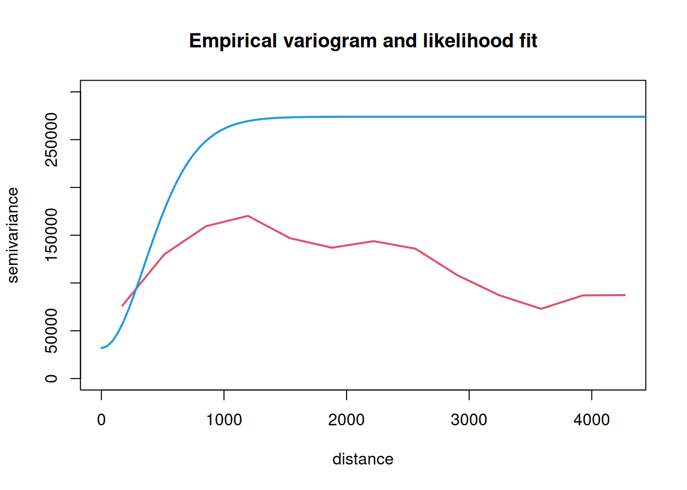
13.5.3 Likelihood estimation of covariograms
If we believe that the process is stationary, and that we have enough data to be able to reliably estimate the mean, then we can evaluate the likelihood associated with the parameters of a given covariance function. We can then attempt to numerically optimise the likelihood. The function geoR::likfit can be used for this purpose.
me.ml=likfit(coords=meuse[,c("x","y")], data=meuse$zinc, cov.model="matern", fix.kappa=FALSE, kappa=me.fit$kappa, # init for kappa ini=me.fit$cov.pars)# inits for sigma^2 and phi
---------------------------------------------------------------
likfit: likelihood maximisation using the function optim.
likfit: Use control() to pass additional
         arguments for the maximisation function.
        For further details see documentation for optim.
likfit: It is highly advisable to run this function several
        times with different initial values for the parameters.
likfit: WARNING: This step can be time demanding!
---------------------------------------------------------------
likfit: end of numerical maximisation.
It is often difficult to numerically maximise the likelihood. In any case, the optimisation process here is not simply trying to find a fit that most closely mimics the empirical semi-variogram.
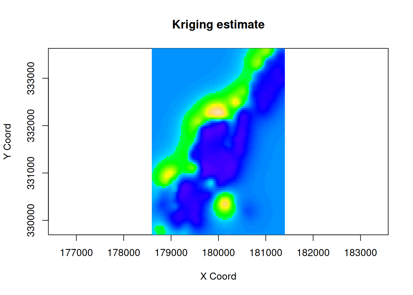
13.6 Kriging in R
Given a valid (estimated) variogram or covariogram function, we can carry out kriging. The function geoR::krige.conv can be used for this purpose. It defaults to ordinary kriging (OK), but it can also do other forms of kriging.
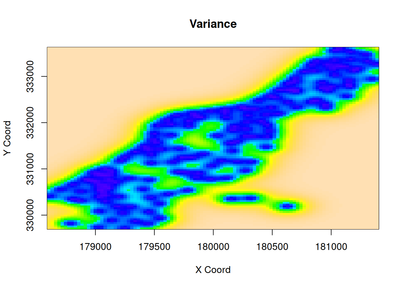
Looking simply at an image of point predictions is potentially misleading, since the predictive uncertainty varies greatly over the kriging area. We can look separately at the variance.
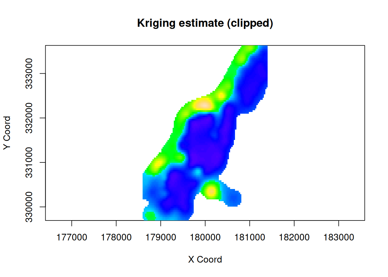
We see that the variance is small in the area where there are plenty of measurements, but increases rapidly in regions where no measurements are available. We can use this information in various ways. One simple approach is to simply clip the kriging estimates when the variance gets too high.