We now consider the problem of modelling and understanding spatial point patterns. Here it is the location of points in space that are of interest. The classic example is that of the location of individual trees within some kind of forest. Typically, the first question of interest is whether or not the points are “truly” randomly distributed in space in some appropriate sense. For this we will need a concept of complete spatial randomness (CSR). It will turn out that the homogeneous Poisson process will be an appropriate stochastic model for CSR, somewhat analogous to the notion of a “white noise” process we have encountered in other areas of spatial and temporal modelling.
17.2 The Poisson process
The Poisson process is often first encountered as a 1-d process, counting occurrences of events in time. However, the complete ordering of the reals leads to approaches to the analysis of the temporal Poisson process that are very specific to the 1-d case, and hence not so relevant in the spatial context. We will therefore skip straight to general Euclidean space, and begin with the important special case of the homogeneous Poisson process.
17.2.1 The homogeneous Poisson process (HPP)
We will define the Poisson process on a spatial domain, \(\mathcal{D}\subseteq\mathbb{R}^d\) (typically, \(d=1,2\), or \(3\)). For any region \(A\subseteq\mathcal{D}\), we can evaluate its volume (or measure), \[
\mu(A) = \int_A \mathrm{d}\mathbf{s}.
\] The Poisson process is a random process, \(N\), which for any (measurable) subset \(A\), defines a non-negative integer value, \(N(A)\), corresponding to the number of events in the region defined by \(A\). The homogeneous Poisson process (HPP) with intensity\(\lambda>0\), has the property that \[
N(A) \sim \text{Pois}\left(\lambda\,\mu(A)\right),
\] and also that for disjoint regions \(A_1,A_2\subseteq\mathcal{D}\) (so that \(A_1\cap A_2=\emptyset\)), \(N(A_1)\) is independent of \(N(A_2)\). The consistency of this definition follows from the fact that the sum of independent Poissons is Poisson with rate the sum of the rates. A HPP is said to be a unit HPP if \(\lambda=1\).
The HPP has a few properties that will be useful to know, and which follow directly from the definition and the properties of the Poisson distribution. First, it is clear that \[
\mathbb{E}[N(A)] = \lambda\, \mu(A),
\] so \(\lambda\) is the area-normalised expectation of the number of events in a region. But expectation is a very crude summary of a very discrete process.
For a (small) region \(\delta A\subseteq\mathcal{D}\) with measure \(\delta a = \mu(\delta A)>0\) we have \[\begin{align*}
\mathbb{P}[N(\delta A)=0] &= 1-\lambda\,\delta a + \mathcal{O}(\delta a^2) \\
\mathbb{P}[N(\delta A)=1] &= \lambda\,\delta a + \mathcal{O}(\delta a^2) \\
\mathbb{P}[N(\delta A)>1] &= \mathcal{O}(\delta a^2) ,
\end{align*}\] and so \(\lambda\) is the hazard (probability normalised by area) of seeing an event at any particular location in space, and the probability of seeing multiple events at the same location is negligible. The HPP has the property that this hazard is independent of the location in space, and this is the sense in which it is homogeneous.
Intuitively, it is now reasonably clear that the HPP has the property that conditional on the number of events being \(n\), then the \(n\) points will be uniformly distributed over the region, \(\mathcal{D}\), since every infinitesimal region, \(\mathrm{d}\mathbf{s}\), has the same hazard, \(\lambda\), of containing a point. Rigorous demonstration of this fact is a little tedious, but the following result gives some insight.
Suppose that \(A\subseteq\mathcal{D}\) is partitioned into \(n\) (mutually disjoint) areas \(A_1,A_2,\ldots,A_n\). Then, conditional on \(N(A)=1\), so that there is exactly one event in the region, \(A\), the probability that this event is in \(A_i\) is \(\mu(A_i)/\mu(A)\). That is, \[
\mathbb{P}[N(A_i)=1|N(A)=1] = \frac{\mu(A_i)}{\mu(A)}.
\] This also follows fairly directly from the definitions. A trivial corollary is that if the areas all have the same measure, \(\mu=\mu(A_i)=\mu(A)/n\), then the probability of being in \(A_i\) is \(1/n\). So, it is clear that conditional on the occurrence of a single event, then this single event is uniformly distributed over \(\mathcal{D}\). It is possible to extend this argument to multiple events, and the upshot is that conditional on the number of events, those events are uniformly and independently distributed over the space. This is why the HPP captures the notion of CSR.
17.2.1.1 Simulating the HPP
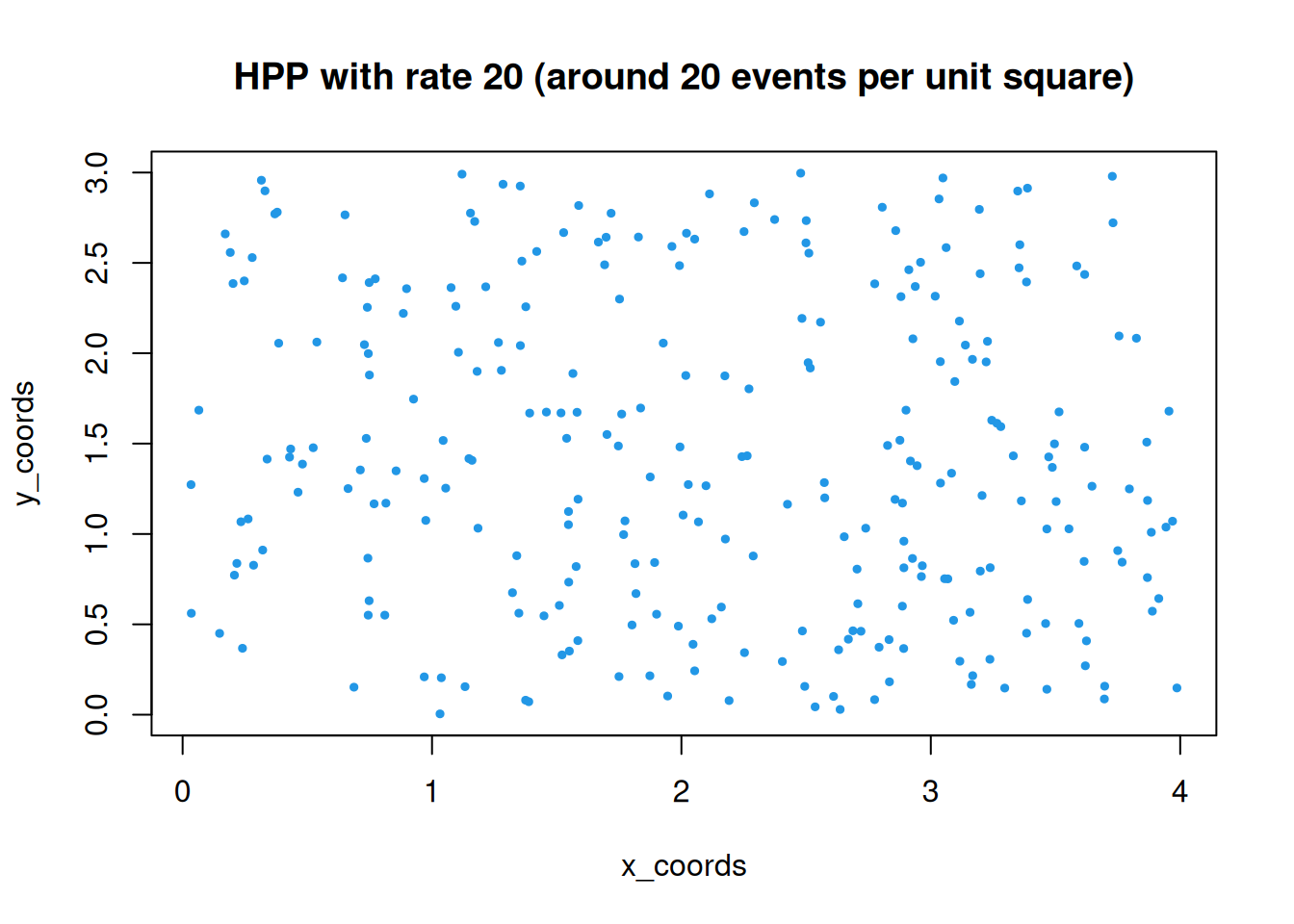
The uniformity property gives us a strategy for simulation. We can first simulate the number of events from the appropriate Poisson distribution, and then distribute those events uniformly in space. This is simplest for rectangular regions. A function to simulate a HPP on a rectangular region (\(d=2\)) is given and illustrated below.
r2dhpp=function(lambda=1, x_max=4, y_max=3){area=x_max*y_maxrate=lambda*arean_events=rpois(1, rate)x_coords=runif(n_events, 0, x_max)y_coords=runif(n_events, 0, y_max)cbind(x_coords, y_coords)}set.seed(7)plot(r2dhpp(20), pch=19, col=4, cex=0.5, main="HPP with rate 20 (around 20 events per unit square)")
For non-rectangular bounded regions, \(\mathcal{D}\), we can use a rejection sampling strategy, where we simulate a HPP on an enclosing rectangle and then keep only the points that lie inside \(\mathcal{D}\).
The HPP will be our reference model for CSR. But what if we are confronted with data that violates CSR? Can we develop models for point processes that are not homogeneous?
17.2.2 The non-homogeneous Poisson process (NHPP)
As the name suggests, the non-homogeneous Poisson process (AKA the inhomogeneous Poisson process) is a Poisson process where the intensity (or event hazard) is allowed to vary over space. Arguing informally, the HPP has the property that \[
\mathbb{P}[N(\mathrm{d}\mathbf{s})=1] = \lambda\,\mu(\mathrm{d}\mathbf{s}),
\] for some fixed \(\lambda>0\). We would like to allow \(\lambda\) to vary in space, so we make \(\lambda\) a function, \[
\lambda: \mathcal{D}\rightarrow \mathbb{R}_{\geq 0},
\] and then desire the property \[
\mathbb{P}[N(\mathrm{d}\mathbf{s})=1] = \lambda(\mathbf{s})\,\mu(\mathrm{d}\mathbf{s}),
\] again, thinking informally of \(\mathrm{d}\mathbf{s}\) as being a volume element located at \(\mathbf{s}\). Due to the nice additive property of the Poisson distribution, it is clear that we will have this property if we define the NHPP via, \[
N(A) \sim \text{Pois}\left( \int_A \lambda(\mathbf{s})\,\mathrm{d}\mathbf{s} \right),
\] for all measurable subsets \(A\subseteq\mathcal{D}\), and it is clear that this reduces to the HPP in the case of a constant \(\lambda(\mathbf{s})=\lambda\). We also have \[
\mathbb{E}[N(A)] = \int_A \lambda(\mathbf{s})\,\mathrm{d}\mathbf{s}.
\]
17.2.2.1 Simulating the NHPP
A number of different approaches can be used for simulating the NHPP, depending on the context. But if \(\mathcal{D}\) is bounded, and an upper bound, \(\lambda^\star\), can be identified for the intensity function (\(\lambda(\mathbf{s})\leq\lambda^\star,\forall\mathbf{s}\in\mathcal{D}\)), then simulation is quite amenable to a simple rejection sampling approach. First identify an enclosing rectangle, \(\mathcal{D}^\star\), for \(\mathcal{D}\), so that \(\mathcal{D}^\star\) is a simple rectangle (or cuboid) such that \(\mathcal{D}\subseteq\mathcal{D}^\star\subseteq\mathbb{R}^d\). Next, simulate a unit HPP on \(\mathcal{D}^\star\times[0,\lambda^\star]\subseteq\mathbb{R}^{d+1}\). For each point in this space, discarding the final coordinate corresponds to projection into \(\mathcal{D}^\star\). Immediately reject any points in this space which do not project into \(\mathcal{D}\). The remaining points will be of the form \((\mathbf{s},z)\) where \(\mathbf{s}\in\mathcal{D}\) and \(z\in[0,\lambda^\star]\). Now reject all points for which \(\lambda(\mathbf{s}) < z\). Then the remaining points will have the property that \(\lambda(\mathbf{s})\geq z\). Standard rejection sampling arguments can be used to see that the projection of these remaining points into \(\mathcal{D}\) will correspond to a NHPP with intensity \(\lambda(\cdot)\).
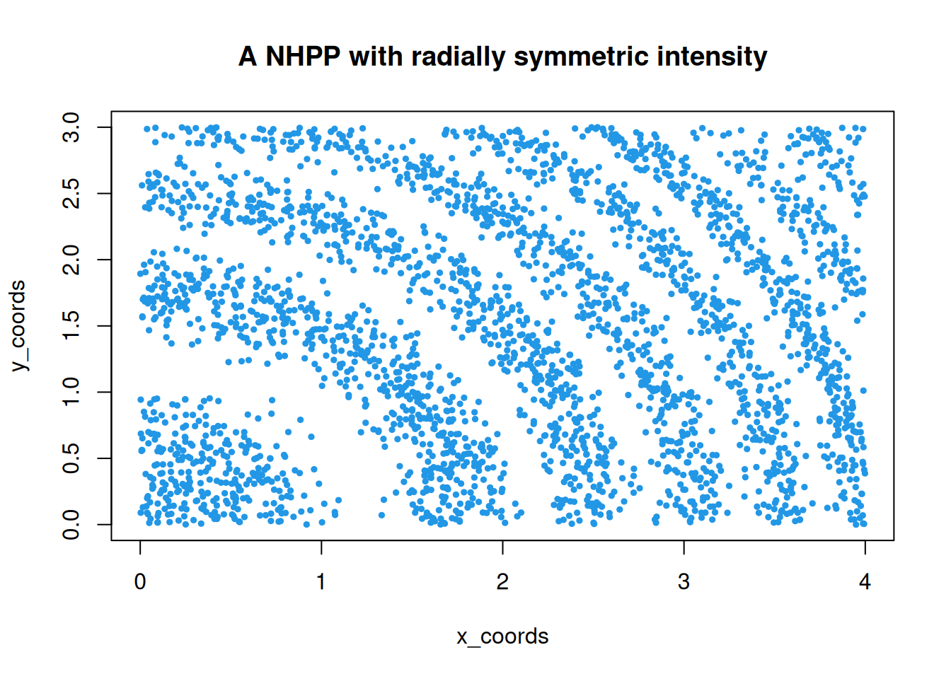
Below is a function to implement this procedure on a simple 2d rectangular region, illustrated on an intensity function with an easily established upper bound.
As we would expect, we see a high density of points in regions where the intensity is high, and very few points in regions where the intensity is low.
17.3 Repulsive processes
The NHPP does not really encapsulate any notion of attraction or repulsion between points. It can be used, in a rather descriptive way, to capture evidence of clustering, suggestive of attraction. But it is not a really a satisfactory model of attractive mechanisms. More fundamentally, it provides no way to model repulsive processes. Satisfactory modelling of repulsive (and attractive) processes requires a fundamentally different approach. Such methods exist but are beyond the scope of this course.
17.4 Empirical measures
When presented with spatial point pattern data, we want to understand it better by thinking about appropriate stochastic models that are consistent with it. Usually the very first question we want to answer is whether the pattern of points is CSR. In other words, is the data consistent with a HPP? We can use some simple empirical measures to begin to think about this.
17.4.1 Quadrat counts
If we divide our region into non-overlapping unit squares (AKA quadrats), then, assuming CSR, we expect the number of events observed in each square to be \(\text{Pois}(\lambda)\), independently of all other squares. We can then look at whether the counts are consistent with this. We don’t have to use quadrats of unit area (and they don’t even need to be square). If we have quadrats of area \(a\), then the counts should be \(\text{Pois}(\lambda a)\) for some intensity \(\lambda\). Assessing the consistency with a Poisson distribution remains the same.
Let’s illustrate with an example, using the spatstat package. The spatstat package is big, but has several vignettes, including a getstart vignette.
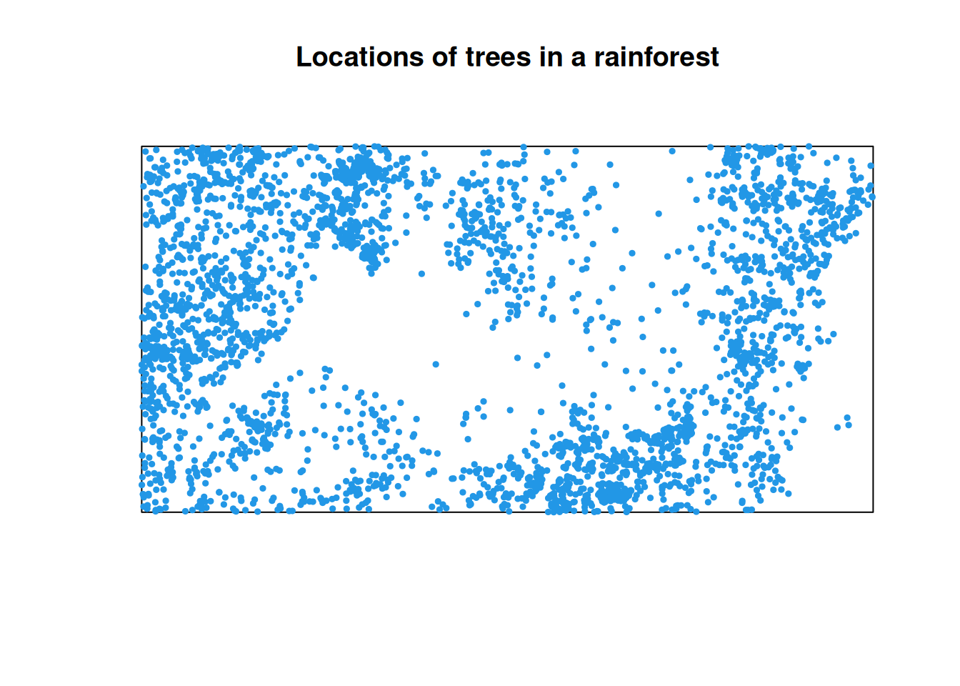
The package contains several point process datasets, using the ppp class (ppp for planar point pattern). spatstat.data::bei are locations of trees in a rainforest.
bei
Planar point pattern: 3604 points
window: rectangle = [0, 1000] x [0, 500] metres
List of 5
 $ window    :List of 4
  ..$ type  : chr "rectangle"
  ..$ xrange: num [1:2] 0 1000
  ..$ yrange: num [1:2] 0 500
  ..$ units :List of 3
  .. ..$ singular  : chr "metre"
  .. ..$ plural    : chr "metres"
  .. ..$ multiplier: num 1
  .. ..- attr(*, "class")= chr "unitname"
  ..- attr(*, "class")= chr "owin"
 $ n         : int 3604
 $ x         : num [1:3604] 11.7 998.9 980.1 986.5 944.1 ...
 $ y         : num [1:3604] 151 430 434 426 415 ...
 $ markformat: chr "none"
 - attr(*, "class")= chr "ppp"
plot(bei, pch=19, cex=0.5, cols=4,
    main="Locations of trees in a rainforest")
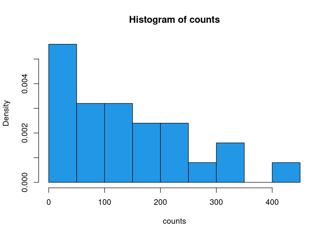
The default plot for ppp objects is fine for most purposes, but the x and y coordinates can be extracted for plotting (and other purposes) as required. It is clear from the plot that this data is not CSR, but we can use spatstat.geom::quadratcount for quadrat counting, which defaults to a \(5\times 5\) grid.
Under CSR these counts should be independent with no spatial dependence. In particular, regarding as a two-way contingency table, the x and y factors should be independent.
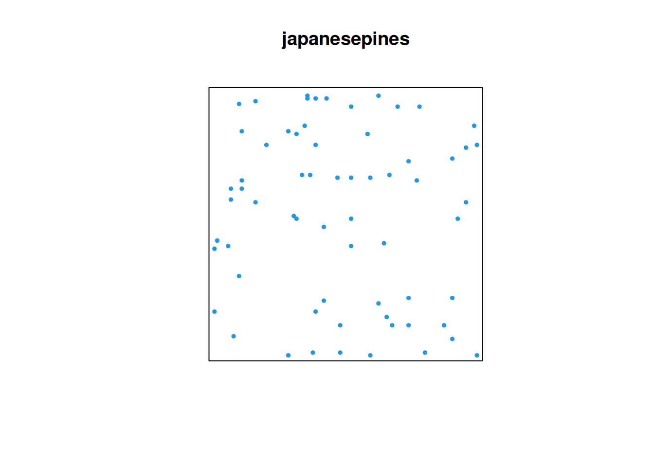
For Poisson data, the mean and variance should be similar, which clearly here they are not. Let’s now switch to spatstat.data::japanesepines, as this is more plausibly CSR.
japanesepines
Planar point pattern: 65 points
window: rectangle = [0, 1] x [0, 1] units (one unit = 5.7 metres)
Number of cases in table: 65
Number of factors: 2
Test for independence of all factors:
    Chisq = 8.593, df = 9, p-value = 0.4757
    Chi-squared approximation may be incorrect
Here there is no evidence that the counts are not independent. Investigating further,
we see that the counts look more Poisson-like, and the mean and variance of the counts turn out to be exactly equal. Exact equality is a bit of a fluke here, but this data seems consistent with CSR.
17.4.2 Kernel smoothing
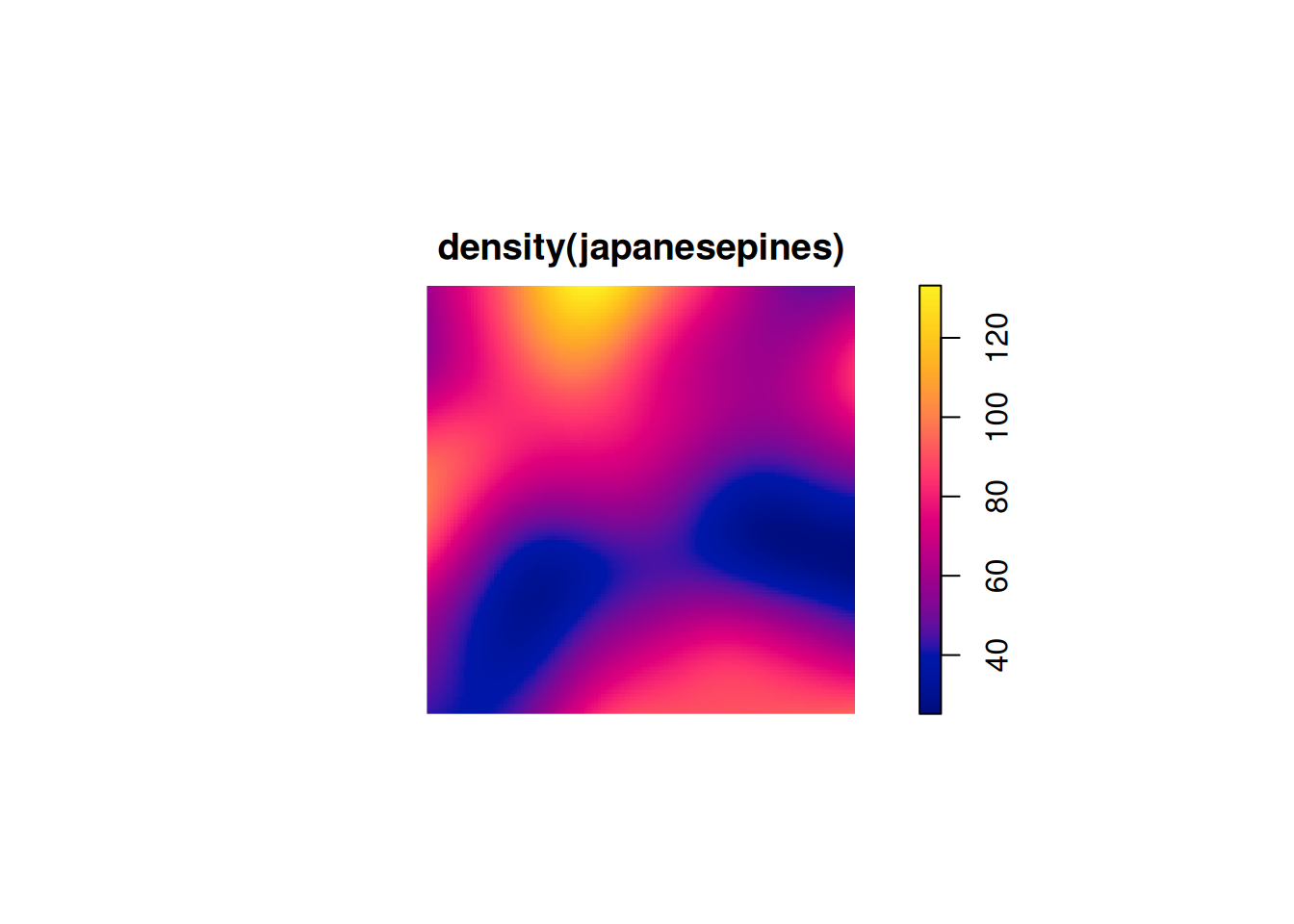
We may be happy to assume that the japanesepines data is CSR, but the bei data clearly isn’t. So the next step may be to wonder whether the bei data is can be modelled with a NHPP. To assess this, we probably want to estimate the intensity function underpinning the data. There are many sophisticated ways that one can approach this problem, but there are also very simple exploratory methods. In particular, one could use a kernel smoothing approach, placing a Gaussian (or other smooth kernel function) at each point location to obtain a smooth field. This is encoded in the function spatstat.explore::density.ppp.
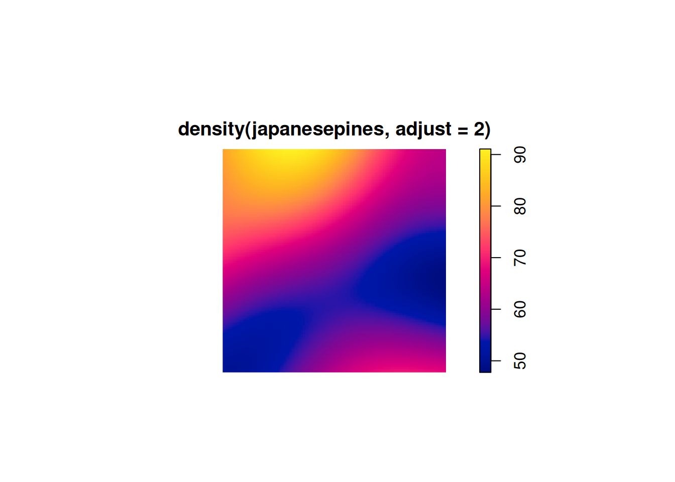
The choice of kernel smoothing bandwidth is crucial for these crude smoothing approaches. The function has some built-in rules-of-thumb which usually work OK. However, it is possible to tweak them, eg. using the adjust argument to increase the level of smoothing.
Quadrat counts are by no means the only way to assess CSR. A descriptive statistic typically referred to as Ripley’s \(K\) function is a very popular way of assessing spatial homogeneity. This is based on the expected number of events within a particular distance of a given point in space. We can use the notation \[
B[\mathbf{s},r] = \left\{\mathbf{s}'\in\mathcal{D}\,\big|\,\Vert\mathbf{s}'-\mathbf{s}\Vert<r\right\},
\] for the ball of radius \(r\) centred on \(\mathbf{s}\). Then, for a stationary point process, \(N\), with intensity \(\lambda\), we define \[
K(r) \equiv \frac{1}{\lambda}\mathbb{E}\big[N(B[\mathbf{s},r])\big],
\] noting that for a stationary process this will be independent of the centre, \(\mathbf{s}\). For the (2-d) HPP we can explicitly compute this, since \(\mu(B[\mathbf{s},r])=\pi r^2\), and hence \[
K(r) = \pi r^2.
\] If we can construct an empirical estimate of \(K(r)\) for a given observed point process dataset, \(\{\mathbf{s}_1,\ldots,\mathbf{s}_n\}\), then we can compare this empirical function against the theoretical prediction. This is somewhat analogous to the use of variograms in geostatistics.
Starting from the definition, if we think of the expectation as an average, we can average the empirically observed number of events within radius \(r\) across all points in the dataset, to posit the empirical estimate \[
\tilde{K}(r) = \frac{1}{n\lambda}\sum_i\sum_{j\not=i} \mathbb{I}(\Vert\mathbf{s}_j-\mathbf{s}_i\Vert < r).
\] In the typical scenario where the true intensity is unknown, it can be estimated as \(\hat{\lambda} = n/D\), where \(D=\mu(\mathcal{D})\) is the area of the study region, to get the estimate \[
\hat{K}(r) = \frac{D}{n^2}\sum_i\sum_{j\not=i} \mathbb{I}(\Vert\mathbf{s}_j-\mathbf{s}_i\Vert < r).
\] This empirical estimate is a reasonable first attempt, but is biased, especially for large \(r\), due to edge effects. That is, close to the boundary of the study region, a ball of radius \(r\) may not be contained within the study region, and so we are unlikely to observe the “expected” number of events within that ball. There are various methods for correcting for this bias, but the details are out of scope for this course.
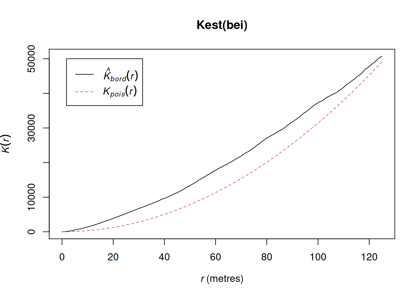
Estimates of the \(K\) function can be computed with spatstat.explore::Kest. For the bei dataset, we get the following plot.
number of data points exceeds 3000 - computing border correction estimate only
This shows an estimated \(K\) function against the theoretical curve for CSR. We see that the estimated curve is consistently and substantially above the theoretical curve. This means that there are more events near to other events than would be expected by chance, and this is suggestive of some kind of clustering.
In contrast, plotting the estimated function for the japanesepines
shows three different estimates all lying quite close to the theoretical curve, especially for small \(r\), where the estimates are more reliable. This is further support for CSR for this data.