As discussed in the previous chapter, we often think of a spatial dataset as being a partial observation of a latent random field that varies continuously in space. It will be helpful to think a bit more carefully about what we mean by random fields and how they should be characterised. Essentially, a random field is a random function whose domain is the spatial domain. That is, for each \(\mathbf{s}\in\mathcal{D}\subset\mathbb{R}^d\) (for some \(d\in\mathbb{N}\), and typically \(d=1,2\) or \(3\)), \(Z(\mathbf{s})\) is a random variable over the sample space \(\mathcal{Z}\subset\mathbb{R}\). A realisation of the random field will be the collection of realisations of the random variables, \(\{z(\mathbf{s})|\mathbf{s}\in\mathcal{D}\}\), and hence a (deterministic) function \(\mathcal{D}\rightarrow\mathcal{Z}\). The variable \(z(\cdot)\) is sometimes said to be regionalised, in order to emphasise its dependence on a continuously varying spatial parameter.
We typically characterise a random variable by its probability distribution, but there is a technical difficulty here, in that we have a distinct (though typically not independent) random quantity at each point in a continuously varying space, and so our random variable is infinite dimensional. Defining probability distributions over such variables is not completely straightforward. Nevertheless, it seems intuitively reasonable that if we are able to specify the joint distribution for any arbitrary finite collection of sites, then this should completely determine the full distribution of the random field. This turns out to be true provided that some reasonable consistency conditions are satisfied. We can define the cumulative distribution function for a finite number of sites as \[ F(z_1,z_2,\ldots,z_n;\mathbf{s}_1,\mathbf{s}_2,\ldots,\mathbf{s}_n) = \mathbb{P}[Z(\mathbf{s}_1)\leq z_1,Z(\mathbf{s}_2)\leq z_2, \ldots,Z(\mathbf{s}_n)\leq z_n]. \] In order to be consistent, \(F(\cdot)\) should be symmetric under a permutation of the site indices (it shouldn’t matter what order the sites are listed), and further, \(F(\cdot)\) should be consistent under marginalisation. That is, \[ F(\infty,z_2,\ldots,z_n;\mathbf{s}_1,\mathbf{s}_2,\ldots,\mathbf{s}_n) = F(z_2,\ldots,z_n;\mathbf{s}_2,\ldots,\mathbf{s}_n). \] Provided an \(F(\cdot)\) can be defined for all \(n\in\mathbb{N}\) in this consistent way, then \(F(\cdot)\) determines the probability distribution of a random field whose finite dimensional distributions are consistent with \(F(\cdot)\). This result is known as Kolmogorov’s extension theorem (AKA the Kolmogorov existence theorem and sometimes as the Kolmogorov consistency theorem).
Not all random fields have finite moments, but when the first moments exist, it is useful to define \(\mu:\mathcal{D}\rightarrow\mathbb{R}\) by \[ \mu(\mathbf{s}) = \mathbb{E}[Z(\mathbf{s})], \quad \forall \mathbf{s}\in\mathcal{D}. \] Similarly, when second moments exist, it is useful to define the covariance function \(C:\mathcal{D}\times\mathcal{D}\rightarrow\mathbb{R}\) by \[ C(\mathbf{s},\mathbf{s}') = \mathbb{C}\mathrm{ov}[Z(\mathbf{s}), Z(\mathbf{s}')], \quad \forall \mathbf{s},\mathbf{s}'\in\mathcal{D}. \] The covariance function must define a positive-definite kernel. This means that for any finite collection of sites, \(\mathbf{s}_1,\mathbf{s}_2,\ldots,\mathbf{s}_n\in\mathcal{D}\), and any \(n\)-vector \(\pmb{\alpha}=(\alpha_1,\alpha_2,\ldots,\alpha_n)^\top\in\mathbb{R}^n\) we must have \[ \sum_{j=1}^n \sum_{k=1}^n \alpha_j\alpha_k C(\mathbf{s}_j,\mathbf{s}_k) \geq 0. \] This is clearly required since \[ \sum_{j=1}^n \sum_{k=1}^n \alpha_j\alpha_k C(\mathbf{s}_j,\mathbf{s}_k) = \mathbb{V}\mathrm{ar}\left[ \sum_{j=1}^n \alpha_j Z(\mathbf{s}_j) \right] \geq 0. \] When first and second moments exist, the field is called a second-order random field.
In the context of time series analysis, we found stationary time series models to be useful building blocks for creating more realistic time series models. The same is true in spatial statistics. For most real, interesting spatial datasets, a stationarity assumption is not reasonable, but a stationary component is often invaluable in the construction of a more appropriate model. A time series model is stationary if its distribution is invariant under a shift in time. A random field is stationary if its distribution is invariant under a shift in space.
A random field is strictly stationary iff \[ F(z_1,z_2,\ldots,z_n;\mathbf{s}_1+\mathbf{h},\mathbf{s}_2+\mathbf{h},\ldots,\mathbf{s}_n+\mathbf{h}) = F(z_1,z_2,\ldots,z_n;\mathbf{s}_1,\mathbf{s}_2,\ldots,\mathbf{s}_n) \] for all finite collections of sites and all shift vectors \(\mathbf{h}\in\mathcal{D}\).
Strict stationarity is an extremely powerful property for a process to have, but just as for time series, a weaker notion of stationarity is useful in practice. A second order random field is weakly stationary (AKA second-order stationary) iff
It is clear that a strictly stationary second-order random field will also be weakly stationary. For weakly stationary random fields we define the function \(C:\mathcal{D}\rightarrow\mathbb{R}\) by \[ C(\mathbf{h}) \equiv C(\mathbf{0},\mathbf{h}). \] This function is the equivalent of the auto-covariance function from time series analysis. In the context of spatial statistics, this function is known as the covariogram. Although we are using \(C\) for two (slightly) different functions, the different domains allow disambiguation. It is clear that the covariogram determines the covariance function, since \(C(\mathbf{s},\mathbf{s}')=C(\mathbf{s}'-\mathbf{s})\). Some basic properties of the covariogram derive directly from properties of covariance.
Sometimes even weak stationarity is too strong a condition. Some processes of interest in geostatistics are not stationary, but do have stationary (and zero mean) increments. A second order process is intrinsically stationary iff
It is clear that weakly stationary processes are intrinsically stationary, but the converse is not true in general. Note that the Wiener process is a simple 1-d example of a random field that is intrinsically stationary but not weakly stationary.
We define the semi-variogram function, \(\gamma:\mathcal{D}\rightarrow\mathbb{R}\) by \[ \gamma(\mathbf{h}) \equiv \frac{1}{2}\mathbb{V}\mathrm{ar}[Z(\mathbf{h})-Z(\mathbf{0})], \] and \(2\gamma(\mathbf{h})\) is the variogram. Note that this use of \(\gamma(\cdot)\) for the semi-variogram is ubiquitous in geostatistics, but somewhat conflicts with its use as an auto-covariance function in time series analysis. Fortunately, it is usually clear from the context which is intended. In the case of an intrinsically stationary process, we have \[ \gamma(\mathbf{h}) = \frac{1}{2}\mathbb{V}\mathrm{ar}[Z(\mathbf{s}+\mathbf{h})-Z(\mathbf{s})], \] where the RHS is independent of \(\mathbf{s}\), and \(\mathbb{V}\mathrm{ar}[Z(\mathbf{s}+\mathbf{h})-Z(\mathbf{s})]\) is the variogram. Note that if intrinsically stationary processes have a mean, then it is constant (say, \(\mathbb{E}[Z(\mathbf{s})]=\mu\)). Unfortunately, the mean and variogram do not completely characterise an intrinsically stationary process, since \(Z(\mathbf{s})\) and \(Z(\mathbf{s})+U\) (where \(U\) is a mean zero random quantity independent of \(Z(\cdot)\)) both have exactly the same increments, the same mean, and the same variogram, but different variances. This problem is usually addressed by fixing (or registering) the value of the field at a single point in space, \(\mathbf{s}_0\in\mathcal{D}\), ie. \(Z(\mathbf{s}_0)\equiv\mu\). This is exactly analogous to fixing the value of a Wiener process to be zero at time zero.
The variogram is a useful concept because it is well-defined for all intrinsically stationary processes, whereas the covariogram is only well-defined for weakly stationary processes. For a process that is weakly stationary, it is clear that the covariogram and variogram are related by \[ \gamma(\mathbf{h}) = C(\mathbf{0}) - C(\mathbf{h}), \quad \forall\mathbf{h}\in\mathbf{D}, \tag{10.1}\] since \(2\gamma(\mathbf{h}) = \mathbb{V}\mathrm{ar}[Z(\mathbf{h})-Z(\mathbf{0})] = C(\mathbf{0})+C(\mathbf{0})-2C(\mathbf{h})\). This allows direct computation of \(\gamma(\cdot)\) from \(C(\cdot)\). To compute \(C(\cdot)\) from \(\gamma(\cdot)\), the stationary variance of the process, \(C(\mathbf{0})\), must also be known. It is worth noting that since \(|C(\mathbf{h})|<C(\mathbf{0})\), \(\gamma(\mathbf{h})\) is bounded above by \(2C(\mathbf{0})\). Consequently, weakly stationary processes cannot have unbounded variograms, and therefore any intrinsically stationary process with an unbounded variogram cannot be weakly stationary.
In the case of a stationary process, it is relatively straightforward to map back and forth between the (semi-)variogram and the covariogram. For an intrinsically stationary process, there is no covariogram, but mapping back and forth between the variogram and the covariance function is often of interest. We will start by computing the variogram from the covariance function, since that is simpler. \[\begin{align*} 2\gamma(\mathbf{h}) &= \mathbb{V}\mathrm{ar}[Z(\mathbf{s}+\mathbf{h})-Z(\mathbf{s})] \\ &= \mathbb{V}\mathrm{ar}[Z(\mathbf{s}+\mathbf{h})] + \mathbb{V}\mathrm{ar}[Z(\mathbf{s})] - 2\mathbb{C}\mathrm{ov}[Z(\mathbf{s}+\mathbf{h}), Z(\mathbf{s})] \end{align*}\] and hence \[ 2\gamma(\mathbf{h}) = C(\mathbf{s}+\mathbf{h}, \mathbf{s}+\mathbf{h}) + C(\mathbf{s}, \mathbf{s}) - 2C(\mathbf{s}+\mathbf{h},\mathbf{s}). \tag{10.2}\] We can use this to compute the variogram from the covariance function. Since the RHS is independent of \(\mathbf{s}\), it will often be convenient to evaluate this at \(\mathbf{s}=\mathbf{0}\), \[ \gamma(\mathbf{h}) = \frac{1}{2}[C(\mathbf{h}, \mathbf{h}) + C(\mathbf{0}, \mathbf{0})] - C(\mathbf{h},\mathbf{0}). \] In general, the variogram is insufficient to determine the covariance function, due to the registration problem. However, if we know the value of the field at some location, then it does become possible to determine the covariance function. It is most convenient if the field is known at the origin, ie. fix \(Z(\mathbf{0})=\mu\). The above equation then simplifies to \[ 2\gamma(\mathbf{h}) = C(\mathbf{h},\mathbf{h}), \] which we can substitute back into Equation 10.2 and rearrange to get \[ C(\mathbf{s}+\mathbf{h}, \mathbf{s}) = \gamma(\mathbf{s}+\mathbf{h})+\gamma(\mathbf{s})-\gamma(\mathbf{h}), \] or alternatively, \[ C(\mathbf{s}',\mathbf{s}) = \gamma(\mathbf{s}')+\gamma(\mathbf{s}) - \gamma(\mathbf{s}'-\mathbf{s}). \tag{10.3}\] So, provided that the field is fixed at the origin, it is actually very straightforward to compute the covariance function from the variogram. It is in this sense that the variogram almost completely characterises an intrinsically stationary random field.
Basic properties of the variogram follow from the definition and the corresponding properties of covariance.
Examples in 1-d can be considered as either having a single spatial dimension, or as being a model for a process in continuous time. We mentioned a few such processes briefly during the time series part of the course.
The Wiener process (mentioned briefly in Chapter 2) is typically defined to have \(W(0)=0\) and \(\mathbb{V}\mathrm{ar}[W(s)-W(t)] = |s-t|,\ s,t\in\mathbb{R}\) (and independent mean zero Gaussian increments). It is therefore intrinsically stationary with semi-variogram \[ \gamma(h) = \frac{1}{2}\mathbb{V}\mathrm{ar}[W(h)-W(0)] = \frac{1}{2}|h|. \] Since it is fixed at zero, we can easily compute its covariance function as \[\begin{align*} C(s, t) &= \gamma(s) + \gamma(t) - \gamma(s-t) \\ &= \frac{1}{2}\left(|s|+|t|-|s-t|\right) \\ &= \min\left\{|s|,|t|\right\}. \end{align*}\]
The Wiener process has a variogram that increases linearly. It is interesting to wonder about processes with a variogram that increases non-linearly, as a fractional power. That is, a process for which \[ \mathbb{V}\mathrm{ar}[Z(t+h)-Z(t)] = |h|^{2H}, \] where the parameter \(H\in(0,1)\) is known as the Hurst index. Clearly the choice \(H=1/2\) gives the Wiener process, but other choices are associated with an intrinsically stationary process known as fractional Brownian motion. Since the variogram is unbounded, we know that the process can not be stationary, but using \[ \gamma(h) = \frac{1}{2}|h|^{2H}, \] if we fix \(Z(0)=0\) we can compute the covariance function as \[ C(s, t) = \frac{1}{2}\left( |s|^{2H} + |t|^{2H} - |s-t|^{2H} \right). \] This is a valid covariance function. It is worth noting that for \(H\not=1/2\), the increments of this process are stationary but not independent. We will revisit this process in Chapter 11.
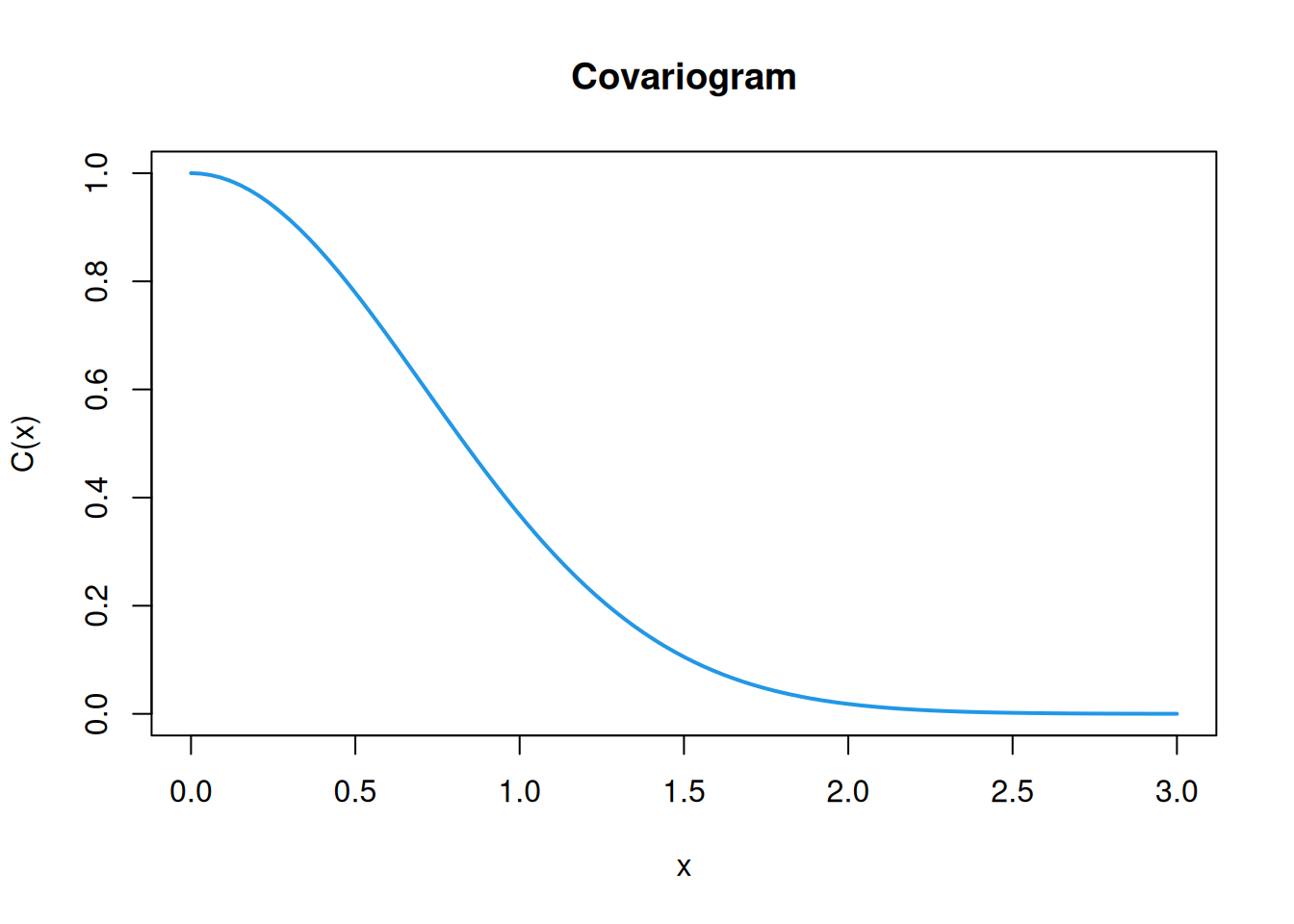
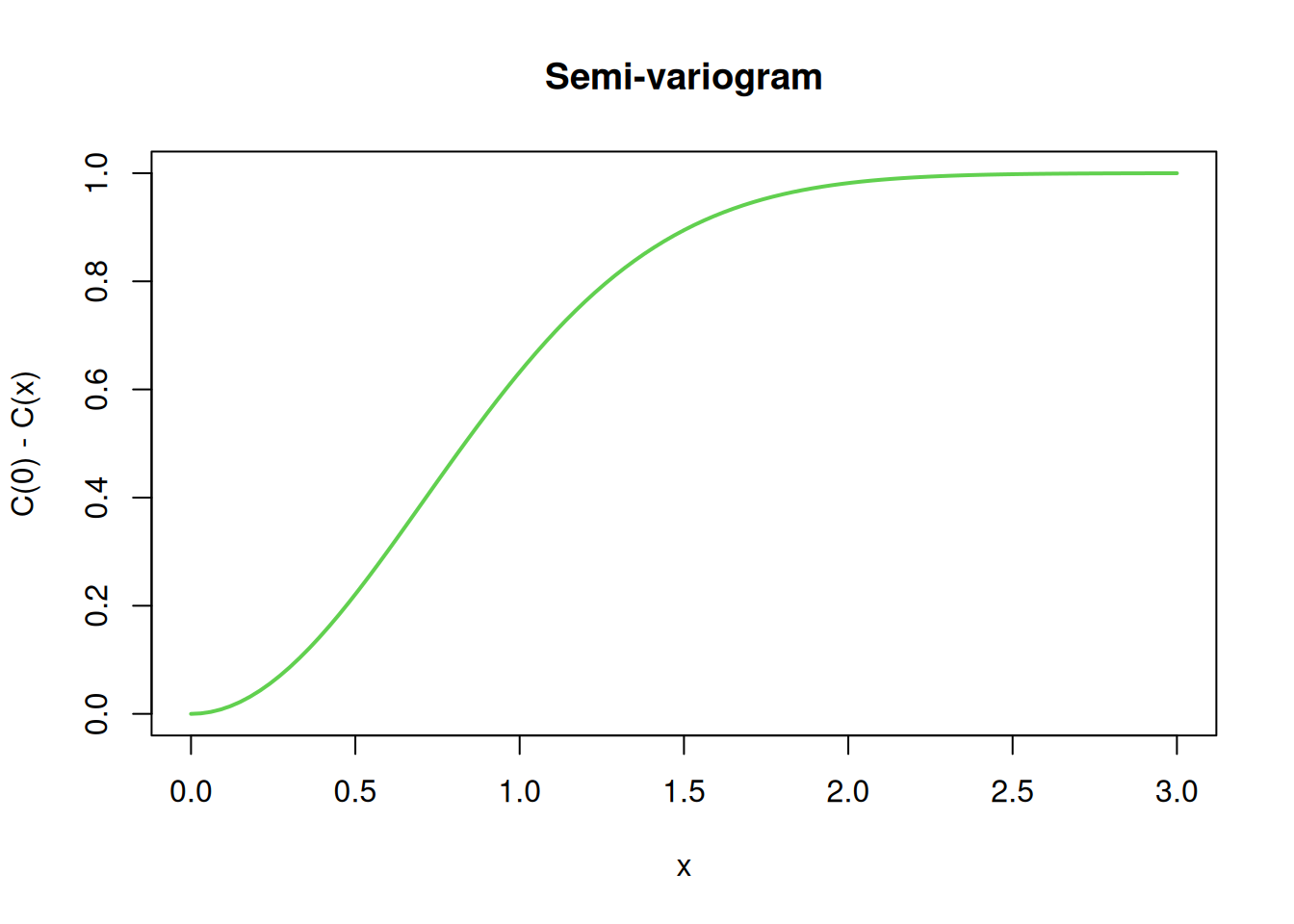
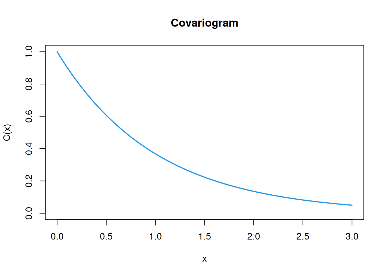
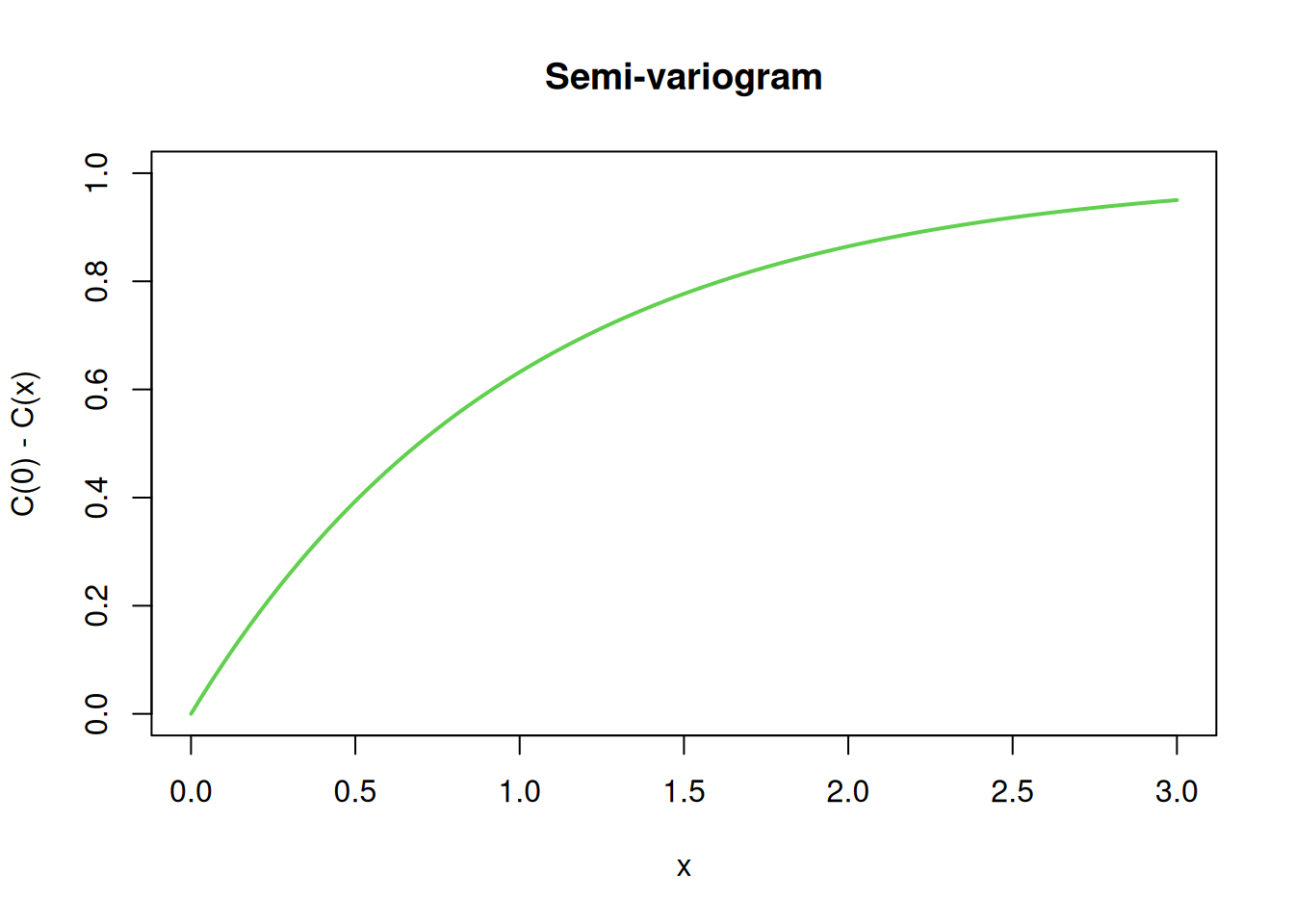
We introduced the OU process in Section 2.3.2.3. By construction this is a Markov process with independent increments, and we showed that for reversion parameter \(\lambda>0\), the process is stationary, with covariogram \[ C(t) = \frac{\sigma^2}{2\lambda}e^{-\lambda|t|}, \] known as the exponential covariance function. We can use Equation 10.1 to compute the semi-variogram as \[ \gamma(t) = \frac{\sigma^2}{2\lambda}(1-e^{-\lambda|t|}). \] So, for \(t>0\), the semi-variogram increases from zero, asymptoting at the stationary variance of the process. Note that not all stationary processes have the stationary variance as the asymptote of the variogram, since not all stationary covariance functions decay away to zero. Plots for the case \(\sigma=1,\ \lambda=\frac{1}{2}\) are given below.
Stationarity (and intrinsic stationarity) is about the invariance of the distribution of a process (or its increments) under a spatial translation. But alone it says nothing about an invariance of the distribution under a spatial rotation. Sometimes this is entirely appropriate. A geospatial process might be invariant under spatial shifts, but have different lengths scales (say) in the North-South versus East-West directions. However, we often want to assume that distributions are rotationally invariant, so that the variogram (and covariogram, if it exists), depends only on the length of the shift vector, and not on its direction. In this case we say that the random field is isotropic. A field or process that is not isotropic is said to be anisotropic.
It is useful to see some examples of isotropic covariogram and variogram families that are known to be valid. There is no need to memorise anything other than the exponential and squared-exponential covariograms.
The exponential covariance function generalises to an isotropic covariagram in the obvious way. However, in the context of spatial statistics, it is often parameterised in terms of its stationary variance, \(\sigma^2>0\), and length scale, \(\phi>0\), to get \[ C(\mathbf{h}) = \sigma^2\exp\{-\Vert\mathbf{h}\Vert/\phi\},\quad \mathbf{h}\in\mathcal{D}. \] Here, \(\Vert\cdot\Vert\) (or \(\Vert\cdot\Vert_2\)) represents the usual Euclidean norm.
\[ C(\mathbf{h}) = \sigma^2\exp\{-(\Vert\mathbf{h}\Vert/\phi)^2\},\quad \mathbf{h}\in\mathcal{D}. \] Although this looks very similar to the exponential covariogram, it has very different properties. Sample paths from processes with an exponential covariance are very rough, but those with a squared-exponential covariogram are very smooth. We will discuss this further later. This covariogram is very often used when a smooth model for a process is required. Plots for the case \(\sigma=\phi=1\) are given below.
The exponential and squared-exponential covariograms are two (important) special cases of a 3-parameter class of covariograms including a smoothness parameter, \(\alpha\in(0,2]\). \[ C(\mathbf{h}) = \sigma^2\exp\{-(\Vert\mathbf{h}\Vert/\phi)^\alpha\},\quad \mathbf{h}\in\mathcal{D}. \]
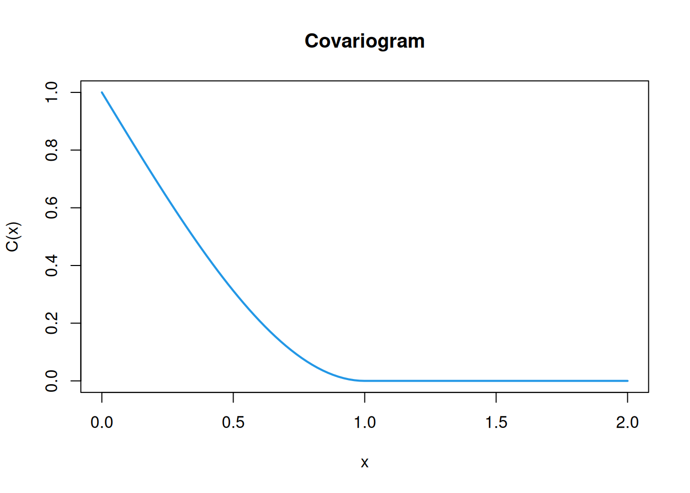
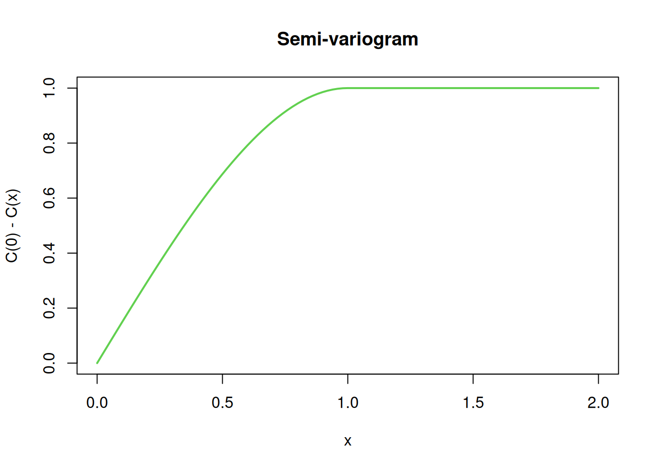
\[ C(\mathbf{h}) = \begin{cases}\displaystyle\sigma^2\left\{ 1 - \frac{3}{2}(\Vert\mathbf{h}\Vert/\phi) + \frac{1}{2}(\Vert\mathbf{h}\Vert/\phi)^3 \right\},&\Vert\mathbf{h}\Vert \leq \phi \\ 0,&\Vert\mathbf{h}\Vert > \phi. \end{cases} \] The compact support of this covariogram can be computationally advantageous, since it leads to sparse covariance matrices. However, it does not have a tunable smoothness parameter. Plots for the case \(\sigma=\phi=1\) are given below.
One of the most popular covariogram families used in geostatistics applications is the Matérn covariance function. It is also parameterised by a stationary variance, a length scale, and a smoothness parameter, conventionally \(\nu > 0\). Again, smoothness increases as \(\nu\) increases. \[ C(\mathbf{h}) = \frac{\sigma^2}{2^{\nu-1}\Gamma(\nu)}\left(\frac{\Vert\mathbf{h}\Vert}{\phi}\right)^\nu K_v\left(\frac{\Vert\mathbf{h}\Vert}{\phi}\right), \] where \(\Gamma(\cdot)\) is the gamma function and \(K_\nu(\cdot)\) is the modified Bessel function of the second kind. There are some important and convenient special cases that may not be apparent from looking at the form of the covariogram.
Every valid isotropic covariogram induces a valid isotropic variogram via Equation 10.1. There are also valid isotropic variograms for fields that are intrinsically stationary but not weakly stationary. For example, the variogram associated with fractional Brownian motion generalises to multiple spatial dimensions as \[ \gamma(\mathbf{h}) = \frac{1}{2}\Vert\mathbf{h}\Vert^{2H},\quad \mathbf{h}\in\mathcal{D}, \] for \(H\in(0,1)\). The choice \(H=1/2\) gives the natural generalisation of the Wiener process to multiple spatial dimensions. Fixing the origin to zero, we can use Equation 10.3 to compute the covariance function as \[ C(\mathbf{s},\mathbf{s}') = \frac{1}{2}\left( \Vert\mathbf{s}\Vert^{2H} + \Vert\mathbf{s}'\Vert^{2H} - \Vert\mathbf{s}-\mathbf{s}'\Vert^{2H} \right),\quad \mathbf{s},\mathbf{s}'\in\mathcal{D}. \] We will use this to define and simulate fractional Brownian motion in 1 and 2 dimensions in subsequent chapters.
There are many ways in which a random field can fail to be isotropic, and it can be difficult to identify appropriate valid variograms in general. However, often an anisotropic process can be made approximately isotropic with a simple distortion of space. Consider, for example, a 2d stationary process for which an exponential kernel is deemed appropriate in both the \(x\) and \(y\) directions, but the variation is twice as fast in the \(x\) direction, so its appropriate length scale is half of that in the \(y\) direction. If we stretch the process in the \(x\) direction by a factor of two, we will then have an isotropic process. Stretching in the \(x\) direction is a simple example of a linear transformation. Any form of anisotropy that can be removed by applying an appropriate linear transformation to the spatial coordinates is referred to as geometric anisotropy. For modelling data generating processes, an appropriate linear transformation can be applied to an isotropic field to get an anisotropic field. When fitting models to data, the inverse linear transformation can be applied to the data coordinates of an anisotropic field to get an isotropic field that can be fit to data more straightforwardly.
A nugget process is an isotropic weakly stationary (Gaussian) random field with mean zero and covariogram \[ C(\mathbf{h}) = \begin{cases} \sigma^2, & \mathbf{h}=0,\\ 0, & \mathbf{h} \not= 0. \end{cases} \] That is, the process is iid (Gaussian) with variance \(\sigma^2\) at every point in space. This process is very closely related to the white noise processes that we considered in the time series part of the course, and many people do refer to this process as a white noise process. However, since it is slightly different to the white noise processes we have previously considered, we will try to refer to this process as a nugget process. Recall that in discrete time, we did refer to a process that is iid Gaussian at every time point as a white noise process, but in continuous time, we said that a white noise process has infinite variance, and covariogram equal to Dirac’s delta function. We will meet such a white noise process again in Chapter 12, so to avoid confusion, we will not overload this term any further.
If we add a nugget process to a weakly stationary random field, we add a jump discontinuity to the covariogram at the origin. Similarly, if we add a nugget process to an intrinsically stationary random field, we cause a jump discontinuity to the variogram at the origin. It is used to model non-spatial variation, or micro-scale variation, on a scale smaller than the sampling scheme. The figure below shows a typical variogram encountered in applied geostatistical modelling. The \(y\)-intercept is called the “nugget”, since it corresponds to the jump discontinuity just discussed. The asymptotic semi-variance (if it exists), is called the “sill”, and the distance at which the sill is (practically) reached is called the “range”, and this relates to the length scale of the process.

More precisely, the nugget variance, \(\sigma^2_\epsilon\) is given by \[ \sigma^2_\epsilon = \lim_{\Vert \mathbf{h}\Vert \rightarrow 0} \gamma(\mathbf{h}). \] The sill is given by \(\lim_{\Vert \mathbf{h}\Vert \rightarrow \infty} \gamma(\mathbf{h})\), and may be infinite, though for a weakly stationary field it will be finite. The range is technically the smallest \(\Vert\mathbf{h}\Vert\) at which the sill is reached, which may be infinite even when the sill is finite. Some pragmatism is often called for here. If the variogram asymptotes gradually to the sill, a common convention is to consider the range to be the smallest \(\Vert\mathbf{h}\Vert\) for which 95% of the sill is reached. The partial sill is the sill minus the nugget, which is sometimes also of interest.