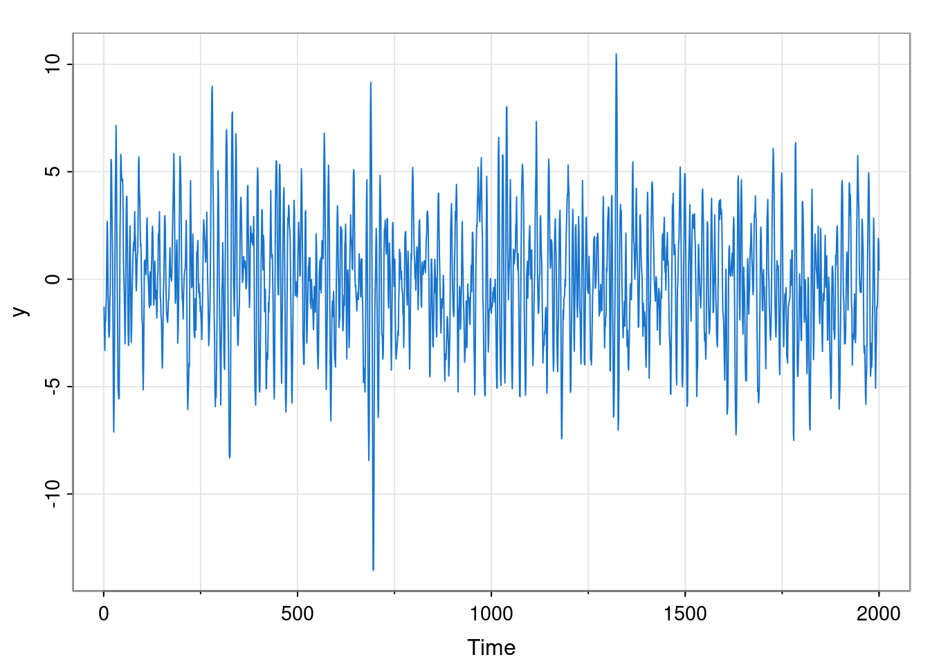
library(astsa)
set.seed(42)
phi = c(1.5, -0.75); sigma = 1; n = 2000; burn = 100
x = filter(rnorm(n+burn, 0, sigma), phi, "rec")[-(1:burn)]
tsplot(x, col=4, cex=0.5, ylab="X_t",
  main=paste0("phi_1=", phi[1], ", phi_2=", phi[2]))
abline(h=0, col=3)
In this chapter we will consider a method for building a flexible class of stationary Gaussian processes for discrete-time real-valued time series. Such processes will rarely be appropriate for directly fitting to real observed time series data, but will be extremely useful for modelling the “residuals” of a time series after taking out some systematic, and/or seasonal effect, and/or detrending in some way. We have seen that such residuals can often be assumed to be mean zero and stationary, but with a non-trivial correlation structure. Autoregressive–moving-average (ARMA) models are good solution to this problem.
An ARMA model is simply the stochastic process obtained by applying an ARMA (or IIR) filter to a Gaussian white noise process. That is, the stochastic process \[\ldots, X_{-2}, X_{-1}, X_0, X_1, X_2, \ldots\] is ARMA\((p,q)\) if it is determined by the filter \[ X_t = \sum_{i=1}^p \phi_i X_{t-i} + \varepsilon_t + \sum_{j=1}^q \theta_j \varepsilon_{t-j}, \tag{3.1}\] applied to iid Gaussian white noise \(\varepsilon_t \sim \mathcal{N}(0,\sigma^2)\), for some fixed \(p\)-vector \(\pmb{\phi}\) and \(q\)-vector \(\pmb{\theta}\). Since the filter is linear, it follows that the ARMA model is a discrete-time Gaussian process. It should be immediately clear that this process generalises the AR(1) and AR(2) processes considered in Chapter 2. However, this connection with the AR(1) and AR(2) should immediately raise questions about stationarity. We have seen that even for these simple special cases, parameters must be carefully chosen in order to ensure that the process is stable and will converge to a stationary distribution. But we have also seen that even in this stable case, if the process is not initialised with draws from the stationary distribution, it will not be stationary, at least until convergence is asymptotically reached.
In the context of time series analysis, we typically want to use ARMA models as a convenient way of describing a stationary discrete-time Gaussian process. We therefore want to restrict our attention to parameter regimes where the process is stable and converges to a stationary distribution. We will need to be careful to check that this is the case. We also assume that the process has been running from \(t=-\infty\), or that it is carefully initialised with draws from the (joint) stationary distribution, so that there is no transient phase of the process that needs to be considered.
At this point it might be helpful to more carefully define stationarity in the context of time series.
A discrete-time stochastic process is strictly stationary iff the joint distribution of \[ X_t,X_{t+1},\ldots X_{t+k} \] is identical to the joint distribution of \[ X_{t+l},X_{t+l+1},\ldots X_{t+l+k}, \quad \forall t,k,l\in\mathbb{Z}. \]
In particular, but not only, it implies that the marginal distribution of \(X_t\) is independent of \(t\). This condition is quite strong, and hard to verify in practice, so there is also a weaker notion of stationarity that is useful.
A discrete-time stochastic process is weakly stationary (AKA second-order stationary) if:
In other words, the mean and variance are constant, and the covariance between two values depends only on the lag. It is clear that (in the case of a process with finite mean and variance) the property of weak stationarity follows from strict stationary, hence the name. However, a Gaussian process is determined by its first two moments, and so for Gaussian processes the concepts of strict and weak stationarity coincide, and we will refer to such processes as being stationary, or not, without needing to qualify.
The sequence \(\gamma_k,\ k\in\mathbb{Z}\) is known as the auto-covariance function of a weakly stationary stochastic process. Note that \(\gamma_{-k}=\gamma_k\). It is often also convenient to work with the corresponding auto-correlation function, \[ \rho_k \equiv \mathbb{C}\mathrm{orr}[X_t,X_{t+k}] = \gamma_k/\gamma_0,\quad \forall k\in\mathbb{Z}. \] Let us now get a better feel for stationary ARMA models by looking at some important special cases.
The Autoregressive model model of order \(p\), denoted AR\((p)\) or ARMA\((p,0)\), is defined by \[ X_t = \sum_{i=1}^p \phi_i X_{t-i} + \varepsilon_t,\quad \varepsilon_t\sim \mathcal{N}(0,\sigma^2),\quad \forall t\in\mathbb{Z}. \tag{3.2}\] The process is determined by fixed \(\pmb{\phi}\in\mathbb{R}^p, \sigma\in\mathbb{R}^+\). We briefly examined the special cases AR(1) and AR(2) in Chapter 2, but we now tackle the general case. It is crucial to notice that, by construction, \(\varepsilon_t\) will be independent of \(X_s\) for \(t>s\), but not otherwise (since then \(\varepsilon_t\) will have been involved in some way in the construction of \(X_s\)). This property also holds in the more general case, and will be repeatedly exploited in the analysis of ARMA models.
The first thing to consider is whether the particular choice of \(\pmb{\phi}\) corresponds to a stable, and hence stationary, model. There are many ways one could try to understand this, but using the same approach as we used in Chapter 2, we can write the model as the \(p\)-dimensional VAR(1) model \[ \begin{pmatrix}X_t\\X_{t-1}\\\vdots\\X_{t-p+1}\end{pmatrix} = \begin{pmatrix} \phi_1&\cdots&\phi_{p-1}&\phi_p\\ 1&\cdots&0&0\\ \vdots&\ddots&\ddots&\vdots\\ 0&\cdots&1&0 \end{pmatrix} \begin{pmatrix}X_{t-1}\\X_{t-2}\\\vdots\\X_{t-p}\end{pmatrix} + \begin{pmatrix}\varepsilon_t\\0\\\vdots\\0\end{pmatrix}. \] If we call the \(p\times p\) autoregressive matrix \(\mathsf{\Phi}\), then we know from our analysis of the stability of VAR(1) models that we will get a (stable) stationary model provided that all of the eigenvalues of \(\mathsf{\Phi}\) lie inside the unit circle in the complex plane. If we attempt to find the eigenvalues by carrying out Laplace expansion on the equation \(|\mathsf{\Phi} -\lambda\mathbb{I}|=0\), we arrive at the polynomial equation \[ \lambda^p - \sum_{k=1}^p \phi_k\lambda^{p-k} = 0. \] So, we want all of the solutions in \(\lambda\) to have modulus less than one.
Aside: Note that we have established a connection between the roots of an arbitrary polynomial and the eigenvalues of a specially constructed matrix. So, if we have a numerical eigenvalue solver at our disposal, we could use it to numerically determine all of the roots of an arbitrary polynomial in a very straightforward way.
If we now make the substitution \(u = \lambda^{-1}\) we get the polynomial equation \[ 1-\sum_{k=1}^p\phi_ku^k=0, \] and so we want all of the solutions to this equation to have modulus greater than one. The polynomial on the LHS of this equation crops up frequently in the analysis of AR models, so it has a name. Our model will be stationary provided that all roots of the characteristic polynomial \[ \phi(u) = 1-\sum_{k=1}^p\phi_ku^k \] have modulus greater than one, and hence lie outside of the unit circle in the complex plane.
We will now assume that we are considering only the stationary case, and try to understand other characteristics of this model. Since we know that it is a stationary Gaussian process, we know that it is characterised by its mean and auto-covariance function. Let’s start with the mean.
It should be obvious, either by symmetry, or by analogy with the AR(1) and AR(2), that the only possible stationary mean for this process is zero. However, it is instructive to explicitly compute it. Taking the expectation of Equation 3.2 gives \[\begin{align*} \mathbb{E}[X_t] &= \sum_{k=1}^p \phi_k \mathbb{E}[X_{t-k}] \\ \Rightarrow \mu &= \sum_{k=1}^p \phi_k\mu \\ \Rightarrow \left(1-\sum_{k=1}^p\phi_k\right)\mu &= 0 \\ \Rightarrow \phi(1)\mu &= 0 \end{align*}\] Now, since we are assuming a stationary process, the roots of \(\phi(u)\) are outside of the unit circle, and hence \(\phi(1)\not=0\), giving \(\mu=0\) as anticipated (in the stationary case).
Next we consider the auto-covariance function.
If we multiply Equation 3.2 by \(X_{t-k}\) for \(k>0\) and take expectations we get \[
\mathbb{E}[X_{t-k}X_t] = \sum_{i=1}^p\phi_i\mathbb{E}[X_{t-k}X_{t-i}],
\] using the fact that \(\mathbb{E}[X_{t-k}\varepsilon_t]=\mathbb{E}[X_{t-k}]\mathbb{E}[\varepsilon_t]=0\). In other words, \[
\gamma_k = \sum_{i=1}^p \phi_i\gamma_{k-i},\quad k>0.
\tag{3.3}\] So, the auto-covariance function satisfies a linear recurrence. We can either use this linear recurrence directly in order to generate auto-covariances, or seek a general solution. But either way, we will need to know \(\gamma_0,\gamma_1,\ldots,\gamma_{p-1}\) in order to initialise the recursion or fix a particular solution. If we consider the above equations for \(k=1,2,\ldots,p\), and remember that \(\gamma_{-k}=\gamma_k\), we have \(p\) equations in the \(p+1\) unknowns \(\gamma_0, \gamma_1,\ldots,\gamma_p\). So, we need one more linear constraint. There are two commonly adopted ways to proceed from here. Either way, it is useful to consider the case \(k=0\). That is, multiply Equation 3.2 by \(X_t\) and take expectations. First we need to compute \[
\mathbb{E}[X_t\varepsilon_t] = \mathbb{C}\mathrm{ov}[X_t,\varepsilon_t] = \mathbb{C}\mathrm{ov}\left[\sum_i \phi_i X_{t-i} + \varepsilon_t, \varepsilon_t\right] = \mathbb{C}\mathrm{ov}[\varepsilon_t,\varepsilon_t]=\mathbb{V}\mathrm{ar}[\varepsilon_t]=\sigma^2.
\] Then we get \[
\gamma_0 = \sum_{i=1}^p\phi_i\gamma_i + \sigma^2.
\] This gives us the \((p+1)\)th equation that we need to solve for \(\gamma_0, \gamma_1,\ldots,\gamma_p\). There is a related but slightly different approach, where we divide Equation 3.3 by \(\gamma_0\) to get \[
\rho_k = \sum_{i=1}^p \phi_i \rho_{k-i}, \quad k=1,2,\ldots,p,
\] which we regard as \(p\) equations in \(p\) unknowns, since we know that \(\rho_0=1\). These are the equations most commonly referred to as the Yule-Walker equations, though conventions vary. But if we adopt this approach we still need to know the stationary variance \(v=\gamma_0\) in order to complete the characterisation of the process. For that we just divide the above equation for \(\gamma_0\) through by \(\gamma_0\) and re-arrange to get \[
v=\gamma_0 = \frac{\sigma^2}{1-\sum_{i=1}^p \phi_i\rho_i}.
\] The above approach to solving for the particular solution of the auto-covariance function using the Yule-Walker equations is very convenient when solving by hand in the case of an AR(1), AR(2) or AR(3), say, but not especially convenient when solving on a computer in the general case. For this it is more convenient to revert to our formulation in terms of a VAR(1) model, with the auto-regressive matrix \(\mathsf{\Phi}\) already described, and innovation variance matrix \[
\mathsf{\Sigma} = \begin{pmatrix}
\sigma^2&0&\cdots&0\\
0&0&\cdots&0\\
\vdots&\vdots&\ddots&\vdots\\
0&0&\cdots&0
\end{pmatrix}.
\] We then know from our analysis in Chapter 2 that the stationary variance matrix is given by the solution, \(\mathsf{V}\), to \[
\mathsf{V} = \mathsf{\Phi} \mathsf{V} \mathsf{\Phi}^\top+ \mathsf{\Sigma},
\] and that there are standard direct methods to solve this discrete Lyapunov equation (eg. netcontrol::dlyap). The first row (or column) of \(\mathsf{V}\) is \(\gamma_0,\gamma_1,\ldots,\gamma_{p-1}\), as required.
Once we have the first \(p\) auto-covariances, we can use Equation 3.3 to generate more auto-covariances, as required. Alternatively, we can seek an explicit solution for \(\gamma_k\) in terms of \(k\) (only), using standard techniques for solving linear recursions. If we seek solution of the form \(\gamma_k = Au^{-k}\) and substitute this in to Equation 3.3 we find that the \(u\) we require are roots of the characteristic polynomial \(\phi(u)\). If we call the roots \(u_1,\ldots,u_p\), then our general solution will be of the form \[ \gamma_k = \sum_{i=1}^p A_iu_i^{-k}, \] and we can use our first \(p\) auto-covariances to determine \(A_1,\ldots,A_p\).
Although it is not strictly necessary, it is often quite convenient to analyse and manipulate ARMA (and other discrete time) models using the backshift operator (AKA the lag operator).
The backshift operator, \(B\), has the property \[Bx_t = x_{t-1}.\]
It follows that \(B^2x_t=BBx_t=Bx_{t-1}=x_{t-2}\), and hence \(B^kx_t=x_{t-k}\). Then, for consistency, we have \(B^{-1}x_t = x_{t+1}\), the forward shift operation, and \(B^0x_t=x_t\), the identity. Since it is a linear operator, it can be manipulated algebraically like other operators. It is very much analogous to the differential operator, \(D\), often used in the analysis of (second-order) ODEs. We can use the backshift operator to simplify the description of an AR\((p)\) model as follows. \[\begin{align*} X_t &= \sum_{i=1}^p \phi_i X_{t-i} + \varepsilon_t\\ \Rightarrow X_t - \sum_{i=1}^p \phi_i X_{t-i} &= \varepsilon_t\\ \Rightarrow X_t - \sum_{i=1}^p \phi_i B^iX_t &= \varepsilon_t\\ \Rightarrow \left(1 - \sum_{i=1}^p \phi_i B^i\right) X_t &= \varepsilon_t\\ \Rightarrow (1 - \sum_{i=1}^p \phi_i B^i) X_t &= \varepsilon_t\\ \Rightarrow \phi(B) X_t &= \varepsilon_t,\\ \end{align*}\] where \(\phi(B)\) is the characteristic polynomial evaluated with \(B\). The linear operator \(\phi(B)\) is known as the autoregressive operator.
We can understand some of the algebraic properties of the backshift operator by first expanding an AR(1) with successive substitution. \[\begin{align*} X_t &= \phi X_{t-1} + \varepsilon_t\\ &= \phi(\phi X_{t-2} +\varepsilon_{t-1}) + \varepsilon_t\\ &= \dots \\ &= \sum_{k=0}^\infty \phi^k \varepsilon_{t-k} \\ &= \sum_{k=0}^\infty \phi^k B^k \varepsilon_t \\ &= \left( \sum_{k=0}^\infty (\phi B)^k\right) \varepsilon_t. \\ \end{align*}\] In other words, the model \[ (1-\phi B)X_t = \varepsilon_t \] is exactly equivalent to the model \[ X_t = (1-\phi B)^{-1} \varepsilon_t, \tag{3.4}\] since \[ (1-\phi B)^{-1} = \sum_{k=0}^\infty (\phi B)^k = 1 + \phi B + \phi^2 B^2 + \cdots. \] For reasons to become clear, Equation 3.4 is known as the MA\((\infty)\) representation of the AR(1) process.
Let’s go back to the AR(2) example considered very briefly in Chapter 2.
library(astsa)
set.seed(42)
phi = c(1.5, -0.75); sigma = 1; n = 2000; burn = 100
x = filter(rnorm(n+burn, 0, sigma), phi, "rec")[-(1:burn)]
tsplot(x, col=4, cex=0.5, ylab="X_t",
main=paste0("phi_1=", phi[1], ", phi_2=", phi[2]))
abline(h=0, col=3)
Although in Chapter 2 we briefly switched to plotting discrete-time series with points (to emphasise the distinction between discrete and cts time), we now revert to the more usual convention of joining successive observations with straight line segments.
This model has \(\phi_1=3/2,\ \phi_2=-3/4, \sigma=1\). In principle this completely characterises the process, but on their own, these parameters are not especially illuminating. The plot suggests that this model is probably stationary, but isn’t especially conclusive, so we should certainly check.
To check by hand, we want to find the roots of the characteristic polynomial by solving the quadratic \[ 1-\phi_1 u-\phi_2 u^2 = 0. \] If we substitute in for \(\phi_1\) and \(\phi_2\) and use the quadratic formula we get \[ u_{1,2} = 1 \pm \mathrm{i}/\sqrt{3}, \] and these obviously have modulus greater than one, so the model is stationary.
To check with a computer, it’s arguably more convenient to see if the eigenvalues of the generator of the equivalent VAR(1) model have modulus less than one.
[1] 0.8660254 0.8660254They both have modulus less than one, so again, we are in the stationary region. We can also check that the roots that we calculated by hand are correct.
1/evals[1] 1-0.5773503i 1+0.5773503iIn fact, R has a built-in polynomial root finder, polyroot, so the simplest approach is to use this function to directly find the roots of the characteristic polynomial.
However, having the VAR(1) generator matrix at our disposal will turn out to be useful, anyway, as we will see shortly.
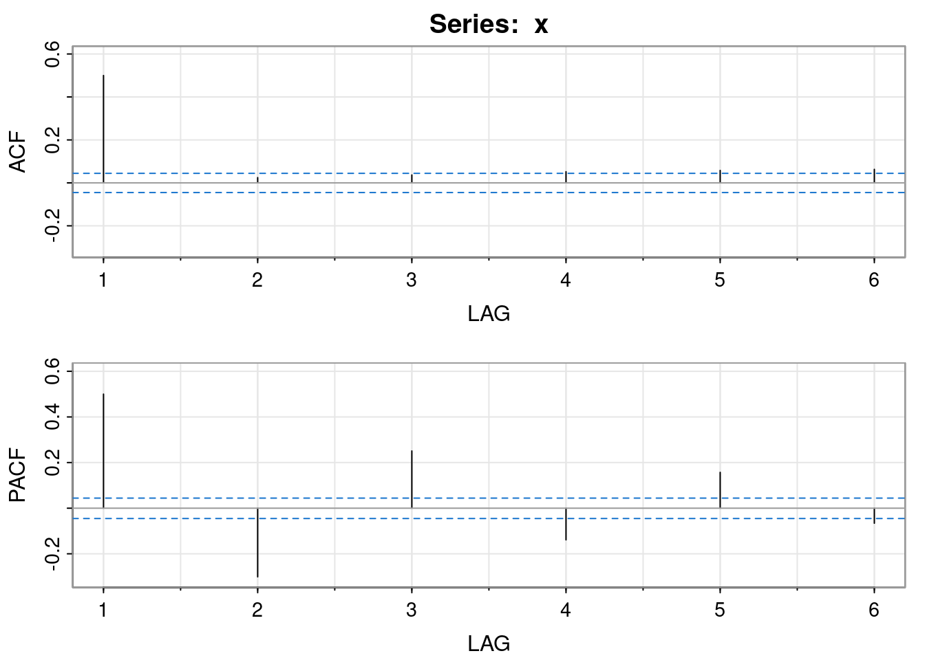
Now that we have established that the process is stationary, attention can focus on the auto-covariance structure. We can start by looking at the empirical ACF of the simulated data.
acf1(x)
 [1]  0.86  0.55  0.18 -0.14 -0.35 -0.41 -0.36 -0.23 -0.08  0.06  0.15  0.18
[13]  0.17  0.12  0.05 -0.02 -0.07 -0.09 -0.09 -0.07 -0.04  0.00  0.03  0.05
[25]  0.05  0.03  0.01  0.00 -0.02 -0.02 -0.02 -0.02 -0.02 -0.02 -0.01  0.00
[37]  0.02  0.03  0.03  0.01  0.00 -0.02 -0.03 -0.04 -0.04 -0.04 -0.02  0.00
[49]  0.02  0.03  0.02  0.00 -0.02 -0.04 -0.04
Given the complex roots of the characteristic polynomial, this oscillatory behaviour in the ACF is to be expected. But what is the true ACF of the model? We know that however we want to compute the auto-covariances, we will need to know the first two, \(\gamma_0=v\) and \(\gamma_1\), in order to initialise the recursion or find a particular solution to the explicit form.
If we want to compute these by hand, we will use some form of the Yule-Walker equations. It is usually easiest to use the auto-correlation form of the Yule-Walker equations. We will look at that approach shortly, but to begin with, it is instructive to examine the approach based on the auto-covariance form. Start with \[\begin{align*} \gamma_0 &= \phi_1\gamma_1 + \phi_2\gamma_2 + \sigma^2 \\ \gamma_1 &= \phi_1\gamma_0 + \phi_2\gamma_1 \\ \gamma_2 &= \phi_1\gamma_1 + \phi_2\gamma_0, \end{align*}\] to get our three equations in three unknowns. To solve these by Gaussian elimination, we can write in the form of an augmented matrix, \[ \left[ \begin{array}{ccc|c} 1&-\phi_1&-\phi_2&\sigma^2\\ -\phi_1&1-\phi_2&0&0\\ -\phi_2&-\phi_1&1&0 \end{array} \right]. \] Substituting in our values gives \[ \left[\begin{array}{ccc|c} 1&-3/2&3/4&1\\ -3/2&7/4&0&0\\ 3/4&-3/2&1&0 \end{array}\right]. \] Row reduction will lead to the first three auto-covariances. I will cheat.
[1] 8.615385 7.384615 4.615385So \(v=\gamma_0=8.62\), \(\gamma_1=7.38\), \(\gamma_2=4.62\).
On a computer, the above approach is not the simplest. Here it is simpler to use our VAR(1) representation and solve for the stationary variance matrix.
         [,1]     [,2]
[1,] 8.615385 7.384615
[2,] 7.384615 8.615385
The first row (or column) of \(\mathsf{V}\) gives the first two auto-covariances. Note that they are the same as we computed above.
Note: According to the documentation for dlyap, it should not be necessary to transpose Phi, but it gives the wrong answer if I don’t. I think this is a bug in either the function or its documentation.
We can check that we do have a good solution by checking that
is close to Sig.
Now that we have the initial auto-covariances we can generate more. If we are on a computer, it may be simplest to just recursively generate them.
initAC = V[1,]
acvf = filter(rep(0,49), c(1.5, -0.75), "rec", init=initAC)
acvf = c(initAC[1], acvf)
acvf[1:20]
[1] 8.6153846 7.3846154 4.6153846 1.3846154 -1.3846154 -3.1153846
[7] -3.6346154 -3.1153846 -1.9471154 -0.5841346 0.5841346 1.3143029
[13] 1.5333534 1.3143029 0.8214393 0.2464318 -0.2464318 -0.5544715
[19] -0.6468835 -0.5544715We can turn these into auto-correlations and overlay them on the empirical ACF of the simulated data set.
acrf = acvf[-1]/acvf[1]
print(acrf[1:20])
[1] 0.85714286 0.53571429 0.16071429 -0.16071429 -0.36160714 -0.42187500
[7] -0.36160714 -0.22600446 -0.06780134 0.06780134 0.15255301 0.17797852
[13] 0.15255301 0.09534563 0.02860369 -0.02860369 -0.06435830 -0.07508469
[19] -0.06435830 -0.04022394acf1(x) [1] 0.86 0.55 0.18 -0.14 -0.35 -0.41 -0.36 -0.23 -0.08 0.06 0.15 0.18
[13] 0.17 0.12 0.05 -0.02 -0.07 -0.09 -0.09 -0.07 -0.04 0.00 0.03 0.05
[25] 0.05 0.03 0.01 0.00 -0.02 -0.02 -0.02 -0.02 -0.02 -0.02 -0.01 0.00
[37] 0.02 0.03 0.03 0.01 0.00 -0.02 -0.03 -0.04 -0.04 -0.04 -0.02 0.00
[49] 0.02 0.03 0.02 0.00 -0.02 -0.04 -0.04
We see that the empirical ACF closely matches the true ACF of the AR(2) model, at least for small lags. In fact, if we just want the auto-correlation function, there is a built-in function to compute it.
          0           1           2           3           4           5
 1.00000000  0.85714286  0.53571429  0.16071429 -0.16071429 -0.36160714
          6           7           8           9          10
-0.42187500 -0.36160714 -0.22600446 -0.06780134  0.06780134
If working by hand, it may be preferable to find an explicit solution for \(\gamma_k\) in terms of \(k\). We know that the solution is of the form \[ \gamma_k = A_1u_1^{-k} + A_2u_2^{-k}, \] where \(u_i\) are the roots of the characteristic equation. We can use \(\gamma_0\) and \(\gamma_1\) to fix \(A_1\) and \(A_2\), since \[\begin{align*} \gamma_0 &= A_1 + A_2 \\ \gamma_1 &= A_1u_1^{-1} + A_2u_2^{-1}, \end{align*}\] and we could write this as the augmented matrix \[ \left[ \begin{array}{cc|c} 1&1&\gamma_0\\ u_1^{-1}&u_2^{-1}&\gamma_1 \end{array} \right]. \] Substituting in our values give \[ \left[ \begin{array}{cc|c} 1&1&8.615\\ 1/(1-\mathrm{i}/\sqrt{3})&1/(1+\mathrm{i}/\sqrt{3})&7.385 \end{array} \right], \] which we can row-reduce to compute \(A_1\) and \(A_2\). Again, I will cheat.
m = matrix(c(1,1, 1/complex(r=1,i=-1/sqrt(3)), 1/complex(r=1,i=1/sqrt(3))),
      ncol=2, byrow=TRUE)
A = solve(m, c(8.615, 7.385))
A
[1] 4.3075-1.066655i 4.3075+1.066655iSo \(A_1=4.31-1.07i\), \(A_2=4.31+1.07i\) are complex conjugates, just as the roots of the characteristic polynomial are. This is to be expected, since \[ \gamma_k = Au^{-k} + \bar{A}\bar{u}^{-k} \] clearly has the property that \(\gamma_k=\bar{\gamma}_k\), and so \(\gamma_k\) is real, as we would hope. To get rid of the imaginary parts, it is convenient to switch to modulus/argument form, putting \(u=re^{\mathrm{i}\theta}\) (\(r>1\)), \(A=se^{\mathrm{i}\psi}\), since then \[\begin{align*} \gamma_k &= sr^{-k}\left[e^{\mathrm{i}(\psi-k\theta)} + e^{-\mathrm{i}(\psi-k\theta)}\right] \\ &= 2sr^{-k}\cos(\psi-k\theta). \end{align*}\] Writing it this way makes it clear that the frequency of the oscillations in the ACF are determined by \(\theta\), the argument of \(u\).
For our example, the frequency is 1/12, and hence the period of the oscillations is 12. We now have everything we need to express our auto-covariance function explicitly. Here is a quick check using R.
 [1]  8.6150000  7.3850000  4.6162500  1.3856250 -1.3837500 -3.1148438
 [7] -3.6344531 -3.1155469 -1.9474805 -0.5845605  0.5837695
Finally, note that we have been simulating data from an AR model by applying a recursive filter to white noise. This is pedagogically instructive, but there is a function in base R, arima.sim that can simulate data from any ARMA model directly (and from a generalisation of ARMA, known as ARIMA).
We have now completely solved for the auto-covariance function of our example process. However, when working by hand it turns out to be significantly simpler to solve directly for the auto-correlation function of the process using the auto-correlation form of the Yule-Walker equations. This isn’t limiting, since if we want the auto-covariance function, we can just multiply through by the stationary variance. Let’s work this through for our current example. Begin with the auto-correlation form of the first Yule-Walker equation: \[ \rho_1 = \phi_1\rho_0+\phi_2\rho_1 = \phi_1+\phi_2\rho_1, \] since \(\rho_0=1\), and so \[ \rho_1 = \frac{\phi_1}{1-\phi_2}, \] and this is true for any AR(2) model. Substituting in for our \(\phi_1\) and \(\phi_2\) gives \(\rho_1=6/7\). But now we know \(\rho_0\) and \(\rho_1\) we have enough information to initialise the Yule-Walker equations, without having to solve a bunch of linear equations (we have, but the system is smaller and simpler, which is generally the case). If we want to know the stationary variance of the process, we will also need to know \(\rho_2\), which we can calculate directly from the 2nd Yule-Walker equation \[ \rho_2 = \phi_1\rho_1 + \phi_2\rho_0 = \frac{3}{2}\times\frac{6}{7}+\frac{-3}{4}\times 1 = \frac{15}{28}. \] We can then compute the stationary variance, \[ \gamma_0 = \frac{\sigma_2}{1-\phi_1\rho_1-\phi_2\rho_2} = 8\frac{8}{13}. \] We can now look for a general solution to either the auto-correlation or auto-covariance function. We will look at the auto-correlation function. There are many ways to proceed here, but from our above analysis, we know that in the case of an AR(2) with complex roots our solution will end up being of the form \[ \rho_k = Ar^{-k}\cos k\theta + Br^{-k}\sin k\theta, \] where \(u = re^{\mathrm{i}\theta}\) and \(A,B\) are real constants that can be determined by \(\rho_0\) and \(\rho_1\). Clearly for any AR(2), \(\rho_0=1\) implies \(A=1\). Then the equation for \(\rho_1\), \[ \rho_1 = r^{-1}\cos\theta + Br^{-1}\sin\theta, \] can be re-arranged for \(B\) as \[ B = \frac{\rho_1 r - \cos\theta}{\sin\theta}. \] For our example, we have \(r=2/\sqrt{3}\), \(\theta=\pi/6\) and \(\rho_1 = 6/7\), so substituting in gives \[ B = \frac{\frac{6}{7}\frac{2}{\sqrt{3}} - \frac{\sqrt{3}}{2}}{\frac{1}{2}} = \frac{\sqrt{3}}{7}, \] leading to full auto-correlation function \[ \rho_k = \left(\frac{\sqrt{3}}{2}\right)^{k} \cos (k\pi/6) + \frac{\sqrt{3}}{7}\left(\frac{\sqrt{3}}{2}\right)^{k}\sin (k\pi/6) \] A quick check with R confirms that we haven’t messed up.
The ACF is a useful characterisation of the way in which correlations decay away with increasing lag. But the ACF of an AR model does not sharply truncate in general, since observations from the distant past do have some (small) influence on the present. However, that influence is “carried” via the intermediate observations. If we knew the intermediate observations, there would be no way for the observations from the distant past to give us any more information about the present. So, for an AR model, it could be useful to understand the correlation between observations that is “left over” after adjusting for the effect of any intermediate observations. This is the idea behind the partial auto-correlation function (PACF).
In the context of stationary Gaussian time series, the partial auto-covariance at lag \(k\) is just the conditional covariance \[ \gamma^\star_k = \mathbb{C}\mathrm{ov}[X_{t-k},X_t|\mathbf{X}_{(t-k+1):(t-1)}]. \] This is well-defined, since we know from multivariate normal theory that the conditional covariance does not actually depend on the observed value of the conditioning variable. Nevertheless, it can sometimes be convenient to explicitly include it in the notation, in which case we could write \[ \gamma^\star_k = \mathbb{C}\mathrm{ov}[X_{t-k},X_t|\mathbf{X}_{(t-k+1):(t-1)}=\mathbf{x}_{(t-k+1):(t-1)}]. \] We can then define the partial auto-correlation at lag \(k\) by \[ \rho^\star_k = \frac{\mathbb{C}\mathrm{ov}[X_{t-k},X_t|\mathbf{X}_{(t-k+1):(t-1)}]}{\mathbb{V}\mathrm{ar}[X_t|\mathbf{X}_{(t-k+1):(t-1)}]} = \frac{\gamma^\star_k}{\mathbb{V}\mathrm{ar}[X_t|\mathbf{X}_{(t-k+1):(t-1)}]}. \] Intuitively, it should be clear that for an AR\((p)\), we will have \(\gamma^\star_k = \rho^\star_k = 0,\ \forall k>p\), since then there will be no remaining influence of the observation from lag \(k\) after conditioning on the intervening observations. We can confirm this, since for \(k>p\), \[\begin{align*} \gamma^\star_k &= \mathbb{C}\mathrm{ov}[X_{t-k},X_t|\mathbf{X}_{(t-k+1):(t-1)}=\mathbf{x}_{(t-k+1):(t-1)}] \\ &= \mathbb{C}\mathrm{ov}\left[\left.X_{t-k},\sum_{i=1}^p\phi_iX_{t-i}+\varepsilon_t\right|\mathbf{X}_{(t-k+1):(t-1)}=\mathbf{x}_{(t-k+1):(t-1)}\right] \\ &= \mathbb{C}\mathrm{ov}\left[\left.X_{t-k},\sum_{i=1}^p\phi_ix_{t-i}+\varepsilon_t\right|\mathbf{X}_{(t-k+1):(t-1)}=\mathbf{x}_{(t-k+1):(t-1)}\right] \\ &= \mathbb{C}\mathrm{ov}\left[\left.X_{t-k},\varepsilon_t\right|\mathbf{X}_{(t-k+1):(t-1)}=\mathbf{x}_{(t-k+1):(t-1)}\right] \\ &= 0. \end{align*}\] Another interesting case is the case \(k=p\), since then \[\begin{align*} \gamma^\star_p &= \mathbb{C}\mathrm{ov}[X_{t-p},X_t|\mathbf{X}_{(t-p+1):(t-1)}=\mathbf{x}_{(t-p+1):(t-1)}] \\ &= \mathbb{C}\mathrm{ov}\left[\left.X_{t-p},\sum_{i=1}^p\phi_iX_{t-i}+\varepsilon_t\right|\mathbf{X}_{(t-p+1):(t-1)}=\mathbf{x}_{(t-p+1):(t-1)}\right] \\ &= \mathbb{C}\mathrm{ov}\left[\left.X_{t-p},\sum_{i=1}^{p-1}\phi_ix_{t-i}+\phi_pX_{t-p}+\varepsilon_t\right|\mathbf{X}_{(t-p+1):(t-1)}=\mathbf{x}_{(t-p+1):(t-1)}\right] \\ &= \mathbb{C}\mathrm{ov}\left[\left.X_{t-p},\phi_pX_{t-p}\right|\mathbf{X}_{(t-p+1):(t-1)}=\mathbf{x}_{(t-p+1):(t-1)}\right] \\ &= \phi_p\mathbb{V}\mathrm{ar}\left[\left.X_{t-p}\right|\mathbf{X}_{(t-p+1):(t-1)}=\mathbf{x}_{(t-p+1):(t-1)}\right], \end{align*}\] and hence \[ \rho^\star_p = \phi_p. \] So, importantly, \(\rho^\star_p\not= 0\) for \(\phi_p\not=0\). It is also clear that \(\gamma^\star_1 = \gamma_1\) and \(\rho^\star_1=\rho_1\), since then there are no intervening observations.
Other partial auto-correlations (\(\rho^\star_2,\ldots,\rho^\star_{p-1}\)) are less obvious, but can be computed using standard multivariate normal theory: \[ \mathbb{C}\mathrm{ov}[X,Y|\mathbf{Z}]=\mathbb{C}\mathrm{ov}[X,Y]-\mathbb{C}\mathrm{ov}[X,\mathbf{Z}]\mathbb{V}\mathrm{ar}[\mathbf{Z}]^{-1}\mathbb{C}\mathrm{ov}[\mathbf{Z},Y]. \] However, in practice they are typically computed by a more efficient method, known as the Durbin-Levinson Algorithm (an application of Levinson recursion), but the details of this are not important for this course.
For the AR(2) model that we have been studying, we can use ARMAacf to compute the PACF as well as the ACF.
         0          1          2          3          4
1.0000000 0.8571429 0.5357143 0.1607143 -0.1607143 [1] 8.571429e-01 -7.500000e-01 1.913000e-15 -7.357691e-16The important things to note are that \(\rho^\star_1 = \rho_1\), \(\rho^\star_2=\phi_2\) and \(\rho^\star_k=0,\ \forall k>2\). Crucially, the PACF truncates at the order of the AR model.
Numerous methods exist to estimate partial auto-correlations empirically, from data. The details need not concern us. We can look at both the ACF and PACF for a given dataset using astsa::acf2. eg. we can apply it to our simulated dataset.
acf2(x, max.lag=10)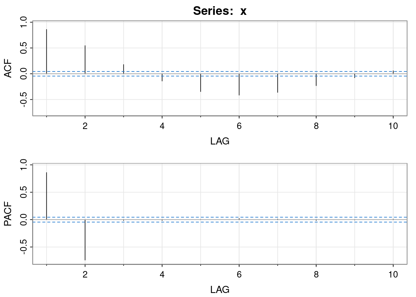
     [,1]  [,2]  [,3]  [,4]  [,5]  [,6]  [,7]  [,8]  [,9] [,10]
ACF  0.86  0.55  0.18 -0.14 -0.35 -0.41 -0.36 -0.23 -0.08  0.06
PACF 0.86 -0.74 -0.01 -0.01 0.00 0.02 0.01 -0.01 -0.01 0.01An MA\((q)\) (or ARMA\((0,q)\)) model is determined by \[ X_t = \varepsilon_t + \sum_{j=1}^q \theta_j \varepsilon_{t-j}, \tag{3.5}\] for white noise \(\varepsilon_t\sim \mathcal{N}(0,\sigma^2)\). In other words, \(X_t\) is the result of applying a FIR convolutional linear filter to white noise. It is immediately clear that (in contrast to the AR model) since white noise is stationary, and the convolutional linear filter being applied is time invariant, that the process will always be stationary, irrespective of the parameters \(\pmb{\theta},\sigma\).
Note that many formula relating to MA processes can be simplified by defining \(\theta_0\equiv 1\), so that \[ X_t = \sum_{j=0}^q \theta_j \varepsilon_{t-j}. \] It is immediately clear via linearity of expectation that the stationary mean is \(\mathbb{E}[X_t]=0\). The stationary variance is also very straightforwardly computed as \[\begin{align*} v=\gamma_0=\mathbb{V}\mathrm{ar}[X_t] &= \sum_{j=0}^q \mathbb{V}\mathrm{ar}[\theta_j\varepsilon_{t-j}] \\ &= \sum_{j=0}^q \theta_j^2\sigma^2 \\ &= \sigma^2 \sum_{j=0}^q \theta_j^2. \end{align*}\] The auto-covariance function is not much more difficult. For \(k>0\) we have \[\begin{align*} \gamma_k &= \mathbb{C}\mathrm{ov}[X_{t-k}, X_t] \\ &= \mathbb{C}\mathrm{ov}\left[\sum_{i=0}^q\theta_i\varepsilon_{t-k-i} , \sum_{j=0}^q\theta_j\varepsilon_{t-j} \right] \\ &= \sum_{i=0}^q\sum_{j=0}^q \theta_i\theta_j\mathbb{C}\mathrm{ov}[\varepsilon_{t-k-i},\varepsilon_{t-j}] \\ &= \sigma^2\sum_{i=0}^q\sum_{j=0}^q \theta_i\theta_j\delta_{k+i,j} \\ &=\sigma^2\sum_{j=k}^q \theta_{j-k}\theta_j, \quad k\leq q \\ &=\sigma^2\sum_{j=0}^{q-k}\theta_j\theta_{j+k}. \end{align*}\] In other words, \[ \gamma_k = \begin{cases} \displaystyle\sigma^2\sum_{j=0}^{q-k}\theta_j\theta_{j+k}, & 0\leq k \leq q, \\ 0, & k>q. \end{cases} \] Note, in particular, that \(\gamma_q = \sigma^2\theta_q \not= 0\) for \(\sigma,\theta_q\not= 0\). Similarly, \[ \rho_k = \begin{cases} \displaystyle\sum_{j=0}^{q-k}\theta_j\theta_{j+k} \Bigg/ \sum_{j=0}^q \theta_j^2, & 0\leq k \leq q, \\ 0, & k>q. \end{cases} \] So, the ACF truncates after lag \(q\).
It can sometimes be useful to write the MA\((q)\) process using backshift notation \[ X_t = \theta(B)\varepsilon_t, \] where \[ \theta(B) = 1 + \sum_{j=1}^q \theta_j B^j \] is known as the moving average operator.
It will be instructive to consider in detail the special case of the MA(1) process \[ X_t = \varepsilon_t + \theta\varepsilon_{t-1} = (1+\theta B)\varepsilon_t. \] The ACF \[ \rho_k = \begin{cases} \frac{\theta}{1+\theta^2},&k=1\\ 0,&k>1 \end{cases} \] has the interesting property that replacing \(\theta\) by \(\theta^{-1}\) leads to exactly the same ACF (try it!). So there are two different values of \(\theta\) that lead to exactly the same ACF. By adjusting the noise variance, \(\sigma^2\) appropriately, we can also ensure that the full auto-covariance function matches up as well. But a mean zero stationary Gaussian process is entirely determined by its auto-covariance function. So there are two different MA(1) models that define exactly the same Gaussian process. This is potentially problematic, especially when it comes to estimating an MA model from data. For reasons to become clear, we should prefer the model with \(|\theta|<1\), and only one of the two models will have that property, so we can use this to rescue us from the potential non-uniqueness problem. We will see how this generalises to general MA\((q)\) process once we better understand why the \(|\theta|<1\) solution is preferred.
We know that the ACF truncates after lag one. Can we say anything about the PACF? Just as we could use successive substitution to turn an AR(1) into an MA\((\infty)\), we can do the same to turn an MA(1) into an AR\((\infty)\). \[\begin{align*} \varepsilon_t &= X_t - \theta \varepsilon_{t-1} \\ &= X_t - \theta (X_{t-1}-\theta\varepsilon_{t-2}) \\ &= \cdots\\ &= X_t + \sum_{j=1}^\infty (-\theta)^jX_{t-j} \end{align*}\] This will converge to an AR\((\infty)\) representation of an MA(1) process provided that \(|\theta|<1\). We say that the process is invertible, in the sense that the MA process can be inverted to an AR process. It may be helpful to write this using backshift notation as \[ \left(1 + \sum_{j=1}^\infty (-\theta)^jB^j\right) X_t = \varepsilon_t. \] This makes perfect sense, since \[ X_t = (1+\theta B)\varepsilon_t \quad\Rightarrow\quad (1+\theta B)^{-1} X_t = \varepsilon_t, \] and \[ (1+\theta B)^{-1} = 1 + \sum_{j=1}^\infty (-\theta)^jB^j. \] So, since (in the invertible case) the MA(1) has a representation as a AR\((\infty)\), and we know that the PACF of a AR\((p)\) truncates after lag \(p\), it is clear that the PACF of the MA(1) will not truncate. You should also be starting to see some duality between AR and MA processes.
We can use R to compute the ACF and PACF of an MA process. eg. For an MA(1) with \(\theta=0.8\):
        0         1         2         3         4         5         6
1.0000000 0.4878049 0.0000000 0.0000000 0.0000000 0.0000000 0.0000000 [1] 0.4878049 -0.3122560 0.2214778 -0.1651935 0.1266695 -0.0987133We can also simulate data, either by applying a convolutional filter to noise, or by using arima.sim.
For an MA(1), we saw that it would be invertible if \(|\theta|<1\). That’s the same as saying that the root of the moving average characteristic polynomial \[ \theta(u) = 1+\theta u \] satisfies \(|u|>1\). This isn’t a coincidence.
For an MA\((q)\), the characteristic polynomial \(\theta(u)\) is of degree \(q\). So, by the fundamental theorem of algebra, we can factor this polynomial in the form \[ \theta(u) = \theta_q\prod_{j=1}^q (u - u_j), \] where \(u_1,\ldots,u_q\) are the roots of \(\theta(u)\). Consequently, we can write \[ \theta(u)^{-1} = \theta_q^{-1}\prod_{j=1}^q (u - u_j)^{-1}, \] so it is reasonably clear that the MA\((q)\) will be invertible if every term of the form \((u-u_j)^{-1}\) has a convergent series expansion. But \[\begin{align*} (u-u_j)^{-1} &= -u_j^{-1}\left(1-\frac{u}{u_j}\right)^{-1}\\ &= -u_j^{-1}\left(1+\frac{u}{u_j}+\frac{u^2}{u_j^2}+\cdots\right) \end{align*}\] will converge for \(|u_j|>1\). Consequently, \(\theta(u)^{-1}\) will have a convergent expansion when all roots of \(\theta(u)\) are outside of the unit circle. This is the condition we will require for the very desirable property of invertibility.
We have seen that a AR\((p)\) process has the property that its PACF will truncate after lag \(p\), but that its ACF does not sharply truncate, but rather decays away geometrically. We have also seen that the MA\((q)\) process has the property that its ACF will truncate after lag \(q\), but that its PACF does not (again, it decays away geometrically). We require the roots of the auto-regressive operator to lie outside of the unit circle in order to ensure stationarity. In fact, this also ensures that the AR process is invertible to an MA process. We also know that although an MA process is always stationary, we nevertheless restrict attention to the case where the roots of the moving average operator lie outside of the unit circle in order to ensure invertibility (and uniqueness). We now turn our attention to the general ARMA process, with both AR and MA components.
We consider the model \[ X_t = \sum_{i=1}^p \phi_i X_{t-i} + \varepsilon_t + \sum_{j=1}^q \theta_j \varepsilon_{t-j}, \] for \(p,q>0\). We could write this with backshift notation as \[ \phi(B)X_t = \theta(B)\varepsilon_t, \] for the appropriately defined auto-regressive and moving-average operators \(\phi(B)\) and \(\theta(B)\), respectively. We assume that the roots of both \(\phi(u)\) and \(\theta(u)\) lie outside of the unit circle, so that the process is stationary and invertible. This means that we can express the ARMA\((p,q)\) model either as the MA\((\infty)\) process \[ X_t = \frac{\theta(B)}{\phi(B)}\varepsilon_t, \] or as the AR\((\infty)\) process \[ \frac{\phi(B)}{\theta(B)}X_t = \varepsilon_t. \] It is then clear that for \(p,q>0\), neither the ACF nor the PACF will sharply truncate.
There is an additional issue that arises for mixed ARMA processes that did not arise in the pure AR or MA case. Start with a pure white noise process \[ X_t = \varepsilon_t \] and apply \((1-\lambda B)\) to both sides (for some fixed \(|\lambda|<1\)) to get \[ X_t = \lambda X_{t-1} + \varepsilon_t - \lambda \varepsilon_{t-1} \] So this now looks like an ARMA(1,1) process. But it is actually the same white noise process that we started off with, as we would find if we tried to compute its ACF, etc. But this is a problem, because there are clearly infinitely many apparently different ways to represent exactly the same stationary Gaussian process. So we are back to having a non-uniqueness/parameter redundancy problem. Again, this will be problematic, especially when we come to think about inferring ARMA models from data. This issue arises whenever \(\phi(u)\) and \(\theta(u)\) contain an identical root. So, in addition to assuming that the roots of \(\phi(u)\) and \(\theta(u)\) all lie outside of the unit circle, we further restrict attention to the case where \(\phi(u)\) and \(\theta(u)\) have no roots in common. If we are presented with an ARMA\((p,q)\) model where \(\phi(u)\) and \(\theta(u)\) do have a root in common, we can just divide out the corresponding linear factor from both in order to obtain an ARMA\((p-1,q-1)\) model that is equivalent (and more parsimonious).
Consider the ARMA(1,1) process \[ X_t = \phi X_{t-1} + \varepsilon_t + \theta\varepsilon_{t-1}, \] for \(|\phi|,|\theta|<1\), \(\varepsilon_t\sim \mathcal{N}(0,\sigma^2)\). For \(k\geq 0\) we can multiply through by \(X_{t-k}\) and take expectations to get \[ \gamma_k = \phi\gamma_{k-1} + \mathbb{C}\mathrm{ov}[X_{t-k},\varepsilon_t] + \theta \mathbb{C}\mathrm{ov}[X_{t-k},\varepsilon_{t-1}]. \] To proceed further it will be useful to know that \[ \mathbb{C}\mathrm{ov}[X_t,\varepsilon_t] = \mathbb{C}\mathrm{ov}[\phi X_{t-1}+\varepsilon_t+\theta\varepsilon_{t-1},\varepsilon_t] = \sigma^2 \] and \[ \mathbb{C}\mathrm{ov}[X_t,\varepsilon_{t-1}] = \mathbb{C}\mathrm{ov}[\phi X_{t-1}+\varepsilon_t+\theta\varepsilon_{t-1},\varepsilon_{t-1}] = \phi\mathbb{C}\mathrm{ov}[X_{t-1},\varepsilon_{t-1}]+\theta\sigma^2 = (\phi+\theta)\sigma^2. \] So now, for \(k=0\) we have \[ \gamma_0 = \phi\gamma_1 + (1+\theta\phi+\theta^2)\sigma^2 \] and for \(k=1\) we have \[ \gamma_1 = \phi\gamma_0 + \theta\sigma^2. \] Solving these gives \[ v=\gamma_0 = \frac{1+2\theta\phi+\theta^2 }{1-\phi^2}\sigma^2 \] and \[ \gamma_1 = \frac{(1+\theta\phi)(\phi+\theta)}{1-\phi^2}\sigma^2. \] For \(k>1\) we have \[ \gamma_k = \phi\gamma_{k-1}, \] and hence \[ \gamma_k = \begin{cases} \displaystyle\frac{1+2\theta\phi+\theta^2 }{1-\phi^2}\sigma^2 & k=0 \\ \displaystyle\frac{(1+\theta\phi)(\phi+\theta)}{1-\phi^2}\phi^{k-1}\sigma^2 & k>0. \end{cases} \] We can also write down the auto-correlation function \[ \rho_k = \frac{(1+\theta\phi)(\phi+\theta)}{1+2\theta\phi+\theta^2}\phi^{k-1},\quad k>0. \] Note that the ACF degenerates to that of a white noise process when \(\theta=-\phi\). This corresponds to the common root redundancy problem discussed above. Note also that the same would happen if \(\phi\theta=-1\), but that our invertibility criterion rules out that possibility.
For concreteness, let’s now study the particular case \(\phi=0.8\), \(\theta=0.6\) using R. We can get R to explicitly compute the ACF and PACF of this model.
        0         1         2         3         4         5         6
1.0000000 0.8931034 0.7144828 0.5715862 0.4572690 0.3658152 0.2926521 [1] 0.89310345 -0.41089371 0.22744126 -0.13276292 0.07888737 -0.04716820We can also simulate data from this model and look at the empirical statistics.