[1] 3243tsplot(y, col=4, main="BoA returns")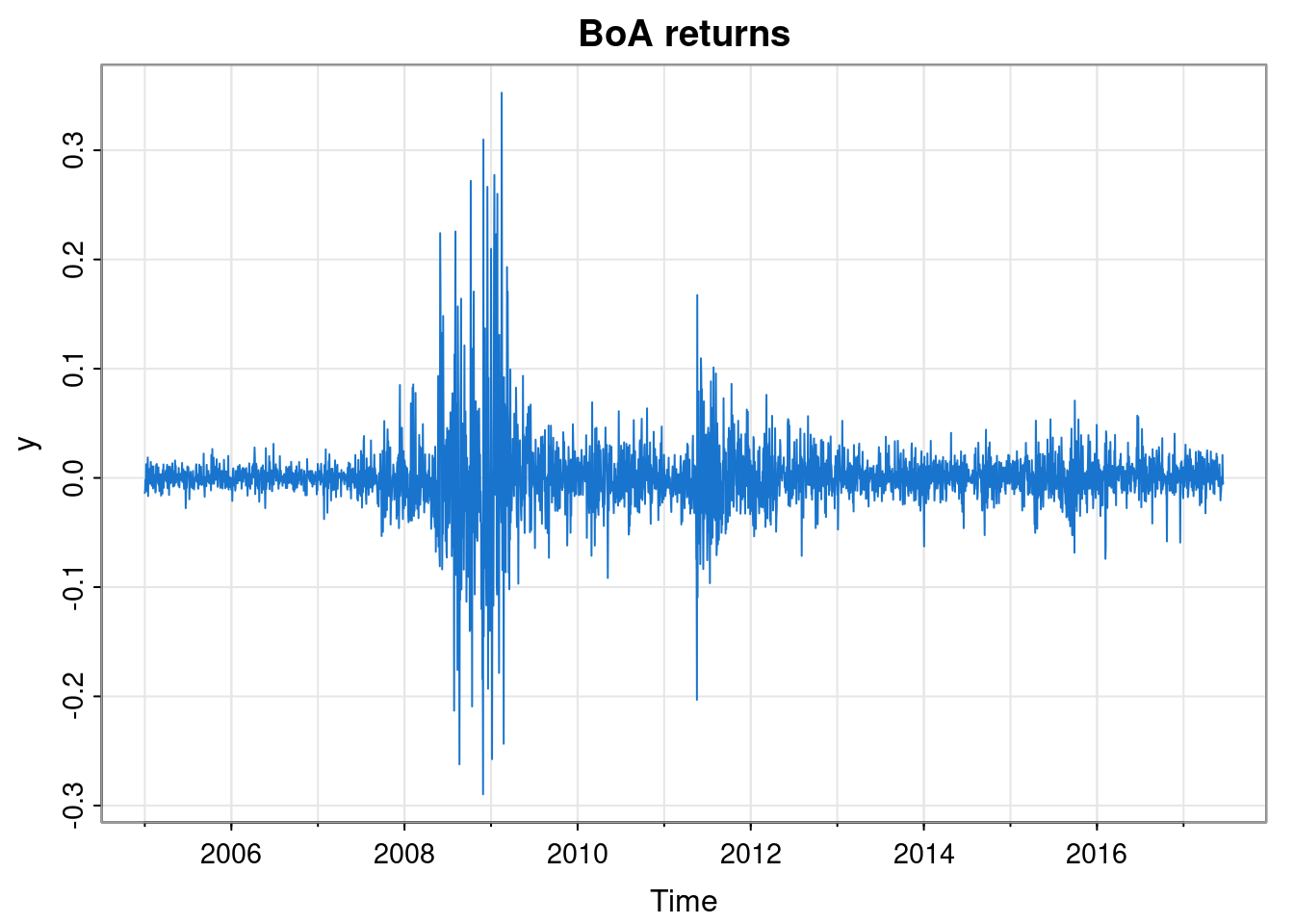
So far we have been assuming that we perfectly observe our time series model. That is, if we have a model for \(X_t\), we observe \(x_t\). However, we are very often in a situation where we have a good model for a (Markov) process \(X_t\), but we are only able to observe some partial or noisy aspects. We call this observation process \(Y_t\) (and to be useful, this observation must depend on \(X_t\) in some way), and hence we only ever observe \(y_t\). The \(X_t\) process remains “hidden”, but we are often able to learn a lot about it from the \(y_t\). This is the idea behind state space modelling. Very often, our hidden process will be a linear Gaussian process like those we have mainly been considering. We will study this case in Chapter 7. It is slightly simpler to start with the case where the hidden process is a finite-state Markov chain. In this case the combined model is referred to as a hidden Markov model.
Our hidden process \(X_0,X_1,\ldots,X_n\) is a Markov chain with state space \(\mathcal{X}=\{1,2,\ldots,p\}\) for some known integer \(p>1\). At time \(t\) the probability that the chain is in each state is described by a (row) vector \[ \pmb{\pi}(t) = (\mathbb{P}[X_t=1],\mathbb{P}[X_t=2],\ldots,\mathbb{P}[X_t=p]). \] The chain is initialised with the vector \(\pmb{\pi}(0)\). The dynamics of the chain are governed by a transition matrix \(\mathsf{P}\), and we use the (usual, but bad, Western) convention that the \((i,j)\)th element corresponds to \(\mathbb{P}[X_{t+1}=j|X_t=i]\). The rows of \(\mathsf{P}\) must then sum to one, and \(\mathsf{P}\) is known as a (right) stochastic matrix. The law of total probability leads to the update rule \[ \pmb{\pi}(t+1) = \pmb{\pi}(t)\mathsf{P}. \tag{6.1}\] It is clear from Equation 6.1 that a distribution \(\pmb{\pi}\) satisfying \[ \pmb{\pi} = \pmb{\pi}\mathsf{P} \] will be stationary. Choosing \(\pmb{\pi}(0)=\pmb{\pi}\) will ensure that the Markov chain is stationary. This is a common choice, but not required. A discrete uniform distribution on the initial states is also commonly adopted, and can sometimes be simpler.
The observation process is \(Y_1, Y_2,\ldots,Y_n\), and will ultimately lead to \(n\) observations \(y_1,y_2,\ldots,y_n\). \(Y_t\) represents some kind of noisy or partial observation of \(X_t\), and so, crucially, is conditionally independent of all other \(X_s\) and \(Y_s\) (\(s\not= t\)) given \(X_t\). In other words, the distribution of \(Y_t\) will depend (directly) only on \(X_t\). The state space, \(\mathcal{Y}\), is largely irrelevant to the analysis. It could be discrete (finite or countable) or continuous. We just need to specify a probability (mass or density) function for the observation which can then be used as a likelihood. We define \[ l_i(y) = \mathbb{P}[Y_t=y|X_t=i], \] but note that this can be replaced with a probability density in the continuous case. Then \(\mathbf{l}(y)\) is a (row) \(p\)-vector of probabilities (or densities) associated with the likelihood of observing some \(y\in\mathcal{Y}\).
For much of this chapter we consider the case where \(\pmb{\pi}(0)\), \(\mathsf{P}\) and \(\mathbf{l}(\cdot)\) are known (though we will consider parameter estimation briefly, later), and we want to use the observations \(y_1,y_2,\ldots,y_n\) to tell us about the hidden Markov chain \((X_0), X_1,X_2,\ldots,X_n\).
As our running example for this chapter, we will look at a financial time series, specifically the daily returns of the Bank of America from 2005 to 2017.
We see that the returns have mean close to zero, as we would expect, but that there are at least two periods of higher volatility - one in 2008/09, and another in 2011. We will use a HMM to automatically segment our time series into regions of high and low volatility.
hist(y[2000:3000], 30, col=4, freq=FALSE,
  main="Region of low volatility")
curve(dnorm(x, 0, 0.015), add=TRUE, col=3, lwd=2)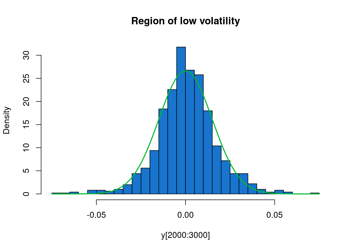
hist(y[1000:1500], 30, col=4, freq=FALSE,
  main="Region of high volatility")
curve(dcauchy(x, 0, 0.025), add=TRUE, col=3, lwd=2)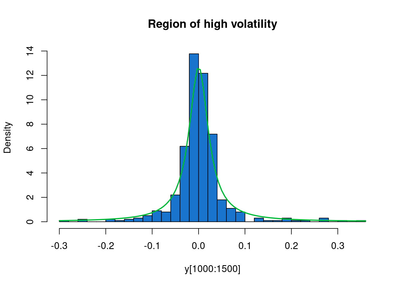
Very informal analysis suggests that we could reasonably model the periods of low volatility as mean zero Gaussian with standard deviation 0.015, and regions of high volatility as Cauchy with scale parameter 0.025.
For our hidden Markov chain, we will suppose that periods of low volatility (\(i=1\)) last for 1,000 days on average, and that periods of high volatility (\(i=2\)) last for 200 days on average, leading to the transition matrix, \[ \mathsf{P} = \begin{pmatrix}0.999&0.001\\0.005&0.995\end{pmatrix}. \] If we further assume \(\pmb{\pi}(0)=(0.5,0.5)\), our model is fully specified.
In the context of state space modelling, the filtering problem is the problem of (sequentially) computing, at each time \(t\), the distribution of the hidden state, \(X_t\), given all data up to time \(t\), \(\mathbf{y}_{1:t}\). That is, we want to compute \[ f_i(t) = \mathbb{P}[X_t=i|\mathbf{Y}_{1:t}=\mathbf{y}_{1:t}],\quad \forall i\in\mathcal{X}, t=0,1,\ldots,n, \] so \(\mathbf{f}(t)\) is the (row) \(p\)-vector of filtered probabilities at time \(t\). We could imagine computing this on-line, as each new observation becomes available. We know that \(\mathbf{f}(0)=\pmb{\pi}_0\), so assume that we know \(\mathbf{f}(t-1)\) for some \(t>0\) and want to compute \(\mathbf{f}(t)\). It is instructive to do this in two steps.
Predict step
We begin by computing \[ \tilde{f}_i(t) = \mathbb{P}[X_t=i|\mathbf{Y}_{1:(t-1)}=\mathbf{y}_{1:(t-1)}],\quad i=1,2,\ldots,p. \] The law of total probability along with conditional independence gives \[\begin{align*} \tilde{f}_i(t) &= \mathbb{P}[X_t=i|\mathbf{Y}_{1:(t-1)}=\mathbf{y}_{1:(t-1)}] \\ &= \sum_{j=1}^p \mathbb{P}[X_t=i|X_{t-1}=j,\mathbf{Y}_{1:(t-1)}=\mathbf{y}_{1:(t-1)}]\mathbb{P}[X_{t-1}=j|\mathbf{Y}_{1:(t-1)}=\mathbf{y}_{1:(t-1)}] \\ &= \sum_{j=1}^p \mathbb{P}[X_t=i|X_{t-1}=j]\mathbb{P}[X_{t-1}=j|\mathbf{Y}_{1:(t-1)}=\mathbf{y}_{1:(t-1)}] \\ &= \sum_{j=1}^p P_{ji}f_j(t-1). \end{align*}\] In other words, \[ \tilde{\mathbf{f}}(t) = \mathbf{f}(t-1)\mathsf{P}. \] This is obviously reminiscent of our fundamental Markov chain update property, Equation 6.1, but does rely on the conditional independence of \(X_t\) and \(\mathbf{Y}_{1:(t-1)}\) given \(X_{t-1}\).
Update step
Now we have pushed our probabilities forward in time, we can condition on our new observation. \[\begin{align*} f_i(t) &= \mathbb{P}[X_t=i|\mathbf{Y}_{1:t}=\mathbf{y}_{1:t}] \\ &= \mathbb{P}[X_t=i|\mathbf{Y}_{1:(t-1)}=\mathbf{y}_{1:(t-1)}, Y_t=y_t] \\ &= \frac{\mathbb{P}[X_t=i|\mathbf{Y}_{1:(t-1)}=\mathbf{y}_{1:(t-1)}]\mathbb{P}[Y_t=y_t|X_t=i,\mathbf{Y}_{1:(t-1)}=\mathbf{y}_{1:(t-1)} ]}{\mathbb{P}[Y_t=y_t|\mathbf{Y}_{1:(t-1)}=\mathbf{y}_{1:(t-1)}]} \\ &= \frac{\mathbb{P}[X_t=i|\mathbf{Y}_{1:(t-1)}=\mathbf{y}_{1:(t-1)}]\mathbb{P}[Y_t=y_t|X_t=i ]}{\mathbb{P}[Y_t=y_t|\mathbf{Y}_{1:(t-1)}=\mathbf{y}_{1:(t-1)}]} \\ &= \frac{\tilde{f}_i(t)l_i(y_t)}{\mathbb{P}[Y_t=y_t|\mathbf{Y}_{1:(t-1)}=\mathbf{y}_{1:(t-1)}]}. \end{align*}\] We could therefore write \[ \mathbf{f}(t) = \frac{\tilde{\mathbf{f}}(t)\circ \mathbf{l}(y_t)}{\mathbb{P}[Y_t=y_t|\mathbf{Y}_{1:(t-1)}=\mathbf{y}_{1:(t-1)}]}, \] where \(\circ\) is the Hadamard (element-wise) product, and the denominator is a scalar normalising constant, and so we could just write \[ \mathbf{f}(t) \propto \tilde{\mathbf{f}}(t)\circ \mathbf{l}(y_t), \] which makes it clearer that we are just re-weighting the results of the predict step according to the likelihood of the observation. We can just compute the RHS and then normalise to get the LHS. Note that we may nevertheless want to keep track of the normalising constant (explained in the next section). If we prefer, we can combine the predict and update steps as \[ \mathbf{f}(t) \propto [\mathbf{f}(t-1)\mathsf{P}]\circ \mathbf{l}(y_t). \] Starting this filtering process off at \(t=1\) and then running it forward to \(t=n\) is the forward part of the forward-backward algorithm.
We can implement the filter by creating a function that advances the algorithm by one step.
We can use this to create the advancement function for our running example as follows.
So advance is now a function that takes the current set of filtered probabilities and an observation and returns the next set of (normalised) filtered probabilities. We can apply this function sequentially to our time series using the Reduce function, which implements a functional fold. If we just want the final set of filtered probabilities, we can call it as follows.
This tells us that we end at a period of low volatility (with very high probability). But more likely, we will want the full set of filtered probabilities, and to plot them over the data in some way.
fpList = Reduce(advance, y, c(0.5, 0.5), acc=TRUE)
fpMat = sapply(fpList, cbind)
fp2Ts = ts(fpMat[2, -1], start=start(y), freq=frequency(y))
tsplot(y, col=4, ylim=c(-0.3, 1))
lines(fp2Ts, col=2, lwd=1.5)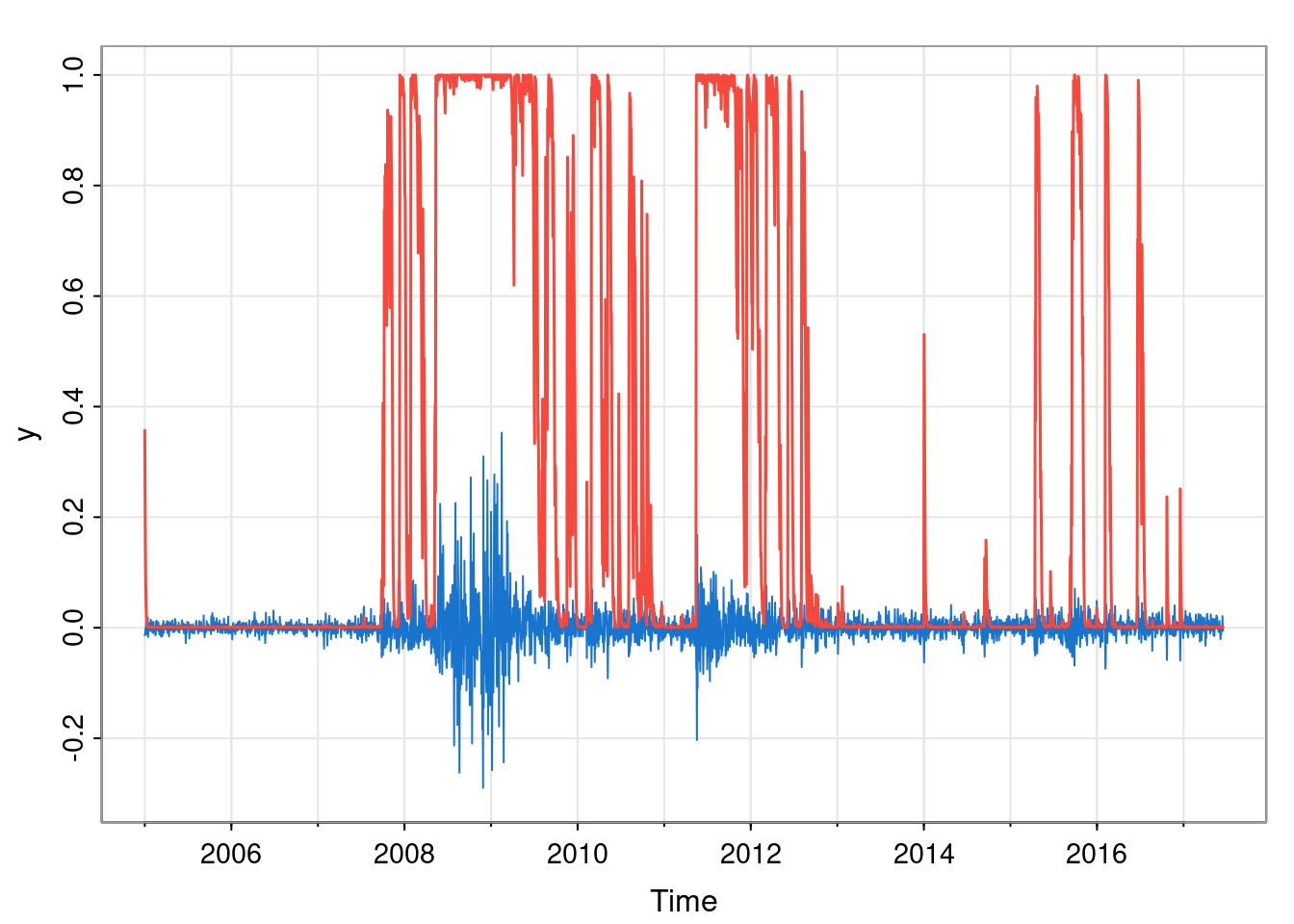
Here we show the filtered probability of being in the high volatility state.
For many reasons (including parameter estimation, to be discussed later), it is often useful to be able to compute the marginal probability (density) of the data, \(\mathbb{P}[\mathbf{Y}_{1:n}=\mathbf{y}_{1:n}]\), not conditioned on the (unknown) hidden states. If we factorise this as \[ \mathbb{P}[\mathbf{Y}_{1:n}=\mathbf{y}_{1:n}] = \prod_{t=1}^n \mathbb{P}[Y_t=y_t|\mathbf{Y}_{1:(t-1)}=\mathbf{y}_{1:(t-1)}], \] we see that the required terms correspond precisely to the normalising constants calculated during filtering. So we can compute the marginal likelihood easily as a by-product of filtering with essentially no additional computation.
In practice, for reasons of numerical stability (in particular, avoiding numerical underflow), we compute the log of the marginal likelihood as \[ \log\mathbb{P}[\mathbf{Y}_{1:n}=\mathbf{y}_{1:n}] = \sum_{t=1}^n \log\mathbb{P}[Y_t=y_t|\mathbf{Y}_{1:(t-1)}=\mathbf{y}_{1:(t-1)}]. \]
We modify our previous function to update the marginal likelihood of the data so far, in addition to the filtered probabilities.
hmmFilterML = function(P, l)
function(fl, y) {
fNew = (fl$f %*% P) * l(y)
ml = sum(fNew)
list(f=fNew/ml, ll=(fl$ll + log(ml)))
}
advance = hmmFilterML(
matrix(c(0.999, 0.001, 0.005, 0.995), ncol=2, byrow=TRUE),
function(y) c(dnorm(y, 0, 0.015), dcauchy(y, 0, 0.025))
)
Reduce(advance, y, list(f=c(0.5, 0.5), ll=0))$f
          [,1]        [,2]
[1,] 0.9989384 0.001061576
$ll
[1] 7971.837This returns the final set of filtered probabilities, as before, but now also the marginal likelihood of the data.
Filtering is great in the on-line context, but off-line, with a static dataset of size \(n\), we are probably more interested in the smoothed probabilities, \[ s_i(t) = \mathbb{P}[X_t=i|\mathbf{Y}_{1:n}=\mathbf{y}_{1:n}], \quad i\in\mathcal{X},\ t=0,1,\ldots,n. \] Now, from the forward filter, we already know the final \[ \mathbf{s}(n) = \mathbf{f}(n). \] So now (for a backward recursion), suppose we already know \(\mathbf{s}(t+1)\) for some \(t<n\), and want to know \(\mathbf{s}(t)\). \[\begin{align*} s_i(t) &= \mathbb{P}[X_t=i|\mathbf{Y}_{1:n}=\mathbf{y}_{1:n}] \\ &= \sum_{j=1}^p \mathbb{P}[X_t=i, X_{t+1}=j|\mathbf{Y}_{1:n}=\mathbf{y}_{1:n}] \\ &= \sum_{j=1}^p \mathbb{P}[X_{t+1}=j|\mathbf{Y}_{1:n}=\mathbf{y}_{1:n}] \mathbb{P}[X_t=i| X_{t+1}=j,\mathbf{Y}_{1:n}=\mathbf{y}_{1:n}] \\ &= \sum_{j=1}^p s_j(t+1) \mathbb{P}[X_t=i| X_{t+1}=j,\mathbf{Y}_{1:t}=\mathbf{y}_{1:t}] \\ &= \sum_{j=1}^p s_j(t+1) \frac{ \mathbb{P}[X_t=i|\mathbf{Y}_{1:t}=\mathbf{y}_{1:t}] \mathbb{P}[X_{t+1}=j| X_{t}=i,\mathbf{Y}_{1:t}=\mathbf{y}_{1:t}]}{ \mathbb{P}[X_{t+1}=j|\mathbf{Y}_{1:t}=\mathbf{y}_{1:t}]} \\ &= \sum_{j=1}^p s_j(t+1) \frac{ f_i(t)P_{ij}}{ \tilde{f}_j(t+1)} \\ &= f_i(t) \sum_{j=1}^p \frac{s_j(t+1)}{ \tilde{f}_j(t+1)} P_{ij} . \end{align*}\] We could write this as \[\begin{align*} \mathbf{s}(t) &= \mathbf{f}(t)\circ\left[\left(\mathbf{s}(t+1)\circ\tilde{\mathbf{f}}(t+1)^{-1}\right)\mathsf{P}^\top\right] \\ &= \mathbf{f}(t)\circ\left[\left(\mathbf{s}(t+1)\circ\left\{\mathbf{f}(t)\mathsf{P}\right\}^{-1}\right)\mathsf{P}^\top\right] . \end{align*}\] So, we can smooth by running backwards using the filtered probabilities from the forward pass.
We can create a function to carry out one step of the backward pass as follows.
We can then create a backward stepping function for our running example with:
We can then apply this to the list of filtered probabilities by requesting that Reduce folds from the right (ie. starts with the final element of the list and works backwards).
spList = Reduce(backStep, fpList, right=TRUE, acc=TRUE)
spMat = sapply(spList, cbind)
sp2Ts = ts(spMat[2, -1], start=start(y), freq=frequency(y))
tsplot(y, col=4, ylim=c(-0.3, 1))
lines(sp2Ts, col=2, lwd=1.5)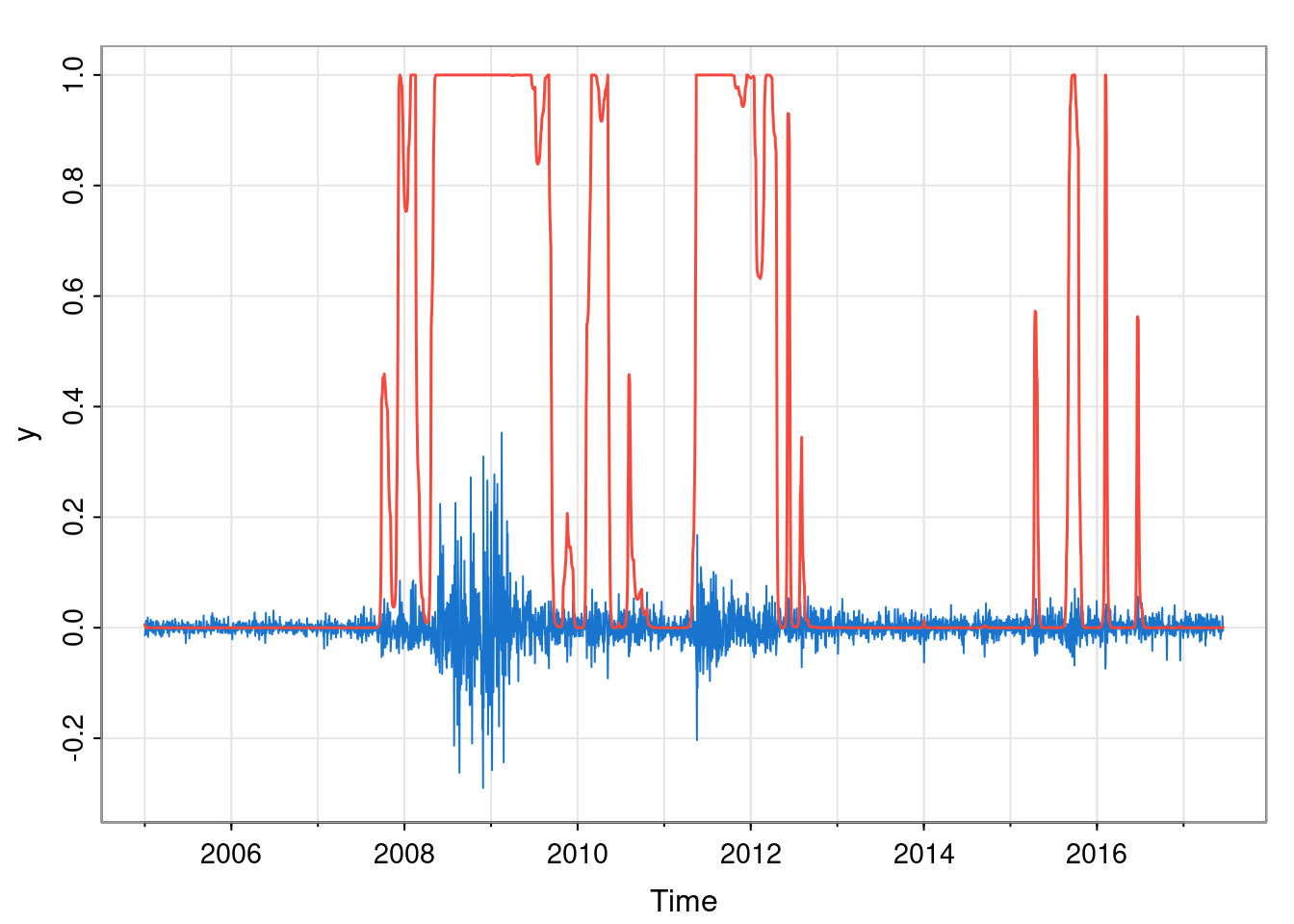
We see that the smoothed probabilities are, indeed, smoother than the filtered probabilities, since the whole time series is used for the marginal classification of each time point.
The smoothed probabilities tell us marginally what is happening at each time point \(t\), but don’t tell us anything about the joint distribution of the hidden states. A good way to get insight into the joint distribution is to generate samples from it. This forms a useful part of many Monte Carlo algorithms for HMMs, including MCMC methods for parameter estimation. So, we want to generate samples from the probability distribution \[ \mathbb{P}[\mathbf{X}_{1:n}|\mathbf{Y}_{1:n}=\mathbf{y}_{1:n}]. \] As with the other problems we have considered in this chapter, naive approaches won’t work. Here, the state space that we are simulating on has size \(p^n\), so we can’t simply enumerate probabilities of possible trajectories. However, we can nevertheless generate exact samples from this distribution by first computing filtered probabilities with a forward sweep, as previously described, but now using a different backward pass.
It is convenient to factorise the joint distribution in a “backwards” manner as \[\begin{align*} \mathbb{P}[\mathbf{X}_{1:n}=\mathbf{x}_{1:n}|\mathbf{Y}_{1:n}=\mathbf{y}_{1:n}] &= \prod_{t=1}^n \mathbb{P}[X_t=x_t|\mathbf{X}_{(t+1):n}=\mathbf{x}_{(t+1):n},\mathbf{Y}_{1:n}=\mathbf{y}_{1:n}] \\ &= \left(\prod_{t=1}^{n-1} \mathbb{P}[X_t=x_t|X_{t+1}=x_{t+1},\mathbf{Y}_{1:t}=\mathbf{y}_{1:t}]\right)\mathbb{P}[X_n=x_n|\mathbf{Y}_{1:n}=\mathbf{y}_{1:n}]. \end{align*}\] Now, we know the final term \(\mathbb{P}[X_n|\mathbf{Y}_{1:n}=\mathbf{y}_{1:n}]=\mathbf{f}(n)\), so we can sample from this to obtain \(x_n\). So now suppose that we know \(x_{t+1}\) for some \(t<n\) and that we want to sample from \[ \mathbb{P}[X_t|X_{t+1}=x_{t+1},\mathbf{Y}_{1:t}=\mathbf{y}_{1:t}]. \] We have \[\begin{align*} \mathbb{P}[X_t=i|X_{t+1}=x_{t+1},\mathbf{Y}_{1:t}=\mathbf{y}_{1:t}] &= \frac{\mathbb{P}[X_t=i|\mathbf{Y}_{1:t}=\mathbf{y}_{1:t}]\mathbb{P}[X_{t+1}=x_{t+1}|X_t=i,\mathbf{Y}_{1:t}=\mathbf{y}_{1:t}]}{\mathbb{P}[X_{t+1}=x_{t+1}|\mathbf{Y}_{1:t}=\mathbf{y}_{1:t}]}\\ &\propto f_i(t)P_{i,x_{t+1}}. \end{align*}\] In other words, the probabilities are proportional to \(\mathbf{f}(t)\circ \mathsf{P}^{(x_{t+1})}\), the relevant column of \(\mathsf{P}\). So, we proceed backwards from \(t=n\) to \(t=1\), sampling \(x_t\) at each step.
We can create a function to carry out one step of backward sampling as follows.
We can then create a backward stepping function for our running example with:
We can then apply this to the list of filtered probabilities.
set.seed(42)
xList = Reduce(backSample, head(fpList, -1),
  init=sample(1:2, 1, prob=tail(fpList, 1)[[1]]),
  right=TRUE, acc=TRUE)
xVec = unlist(xList)
xTs = ts(xVec[-1], start=start(y), freq=frequency(y))
tsplot(y, col=4, ylim=c(-0.3, 1))
lines(xTs-1, col=2, lwd=1.5)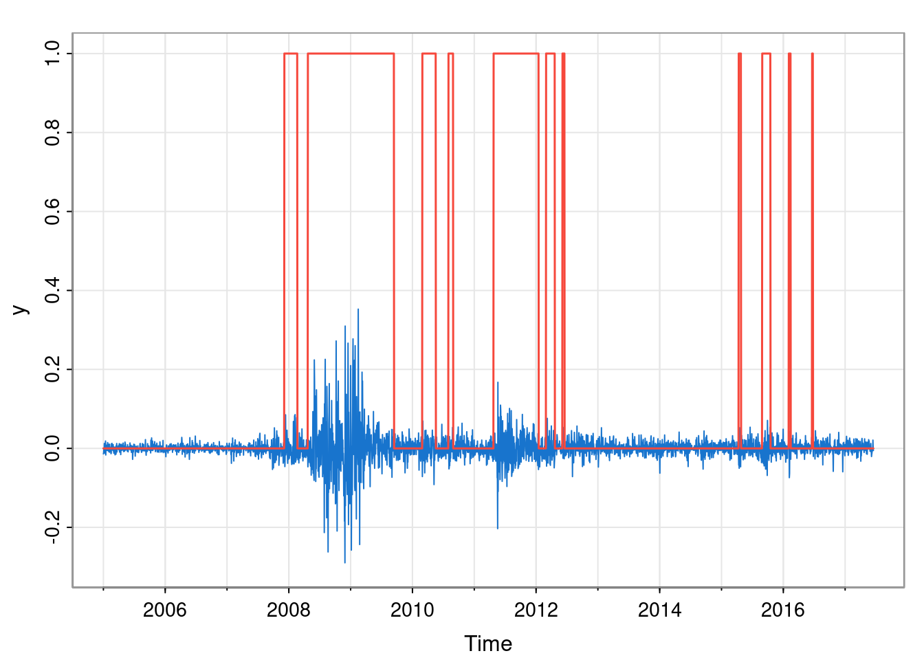
This gives us one sample from the joint conditional distribution of hidden states. Of course, every time we repeat this process we will get a different sample. Studying many such samples gives us a Monte Carlo method for understanding the joint distribution. We do not have time to explore this in detail here.
We have so far assumed that the HMM is fully specified, and that there are no unknown parameters (other than the hidden states). Of course, in practice, this is rarely the case. There could be unknown parameters in either or both of the transition matrix or observation likelihoods, for example. There are many interesting Bayesian approaches to this problem, but for this course we focus on maximum likelihood estimation.
We have seen how we can use the forward filtering algorithm to compute the marginal model likelihood. But evaluation requires a fully specified model, and therefore depends on any unknown parameters. If we call the unknown parameters \(\pmb{\theta}\), then the marginal likelihood is actually the likelihood function, \(\ell(\pmb{\theta};\mathbf{y})\). Maximum likelihood approaches to inference seek to maximise this as a function of \(\pmb{\theta}\). There is a very efficient iterative algorithm for this based on the EM algorithm, which in the context of HMMs, is known as the Baum-Welch algorithm. The details are not relevant to this course, however, so we will just look at generic numerical maximisation approaches.
For our running example, we will assume that we are happy with our specification of the transition matrix for the hidden states, but that we are not so sure about the appropriate scale parameters to use in our observation model. We will carry out ML inference for these two parameters. First, define a function that returns the marginal likelihood for a given vector of scale parameters.
mll = function(theta) {
  advance = hmmFilterML(
    matrix(c(0.999, 0.001, 0.005, 0.995), ncol=2, byrow=TRUE),
    function(yt)
      c(dnorm(yt, 0, theta[1]), dcauchy(yt, 0, theta[2]))
  )
  Reduce(advance, y, list(f=c(0.5, 0.5), ll=0))$ll
}

mll(c(0.015, 0.025))
[1] 7971.837This works, and returns the likelihood we previously obtained when evaluated at our original guess. Can we do better than this? Let’s see if optim can find anything better.
$par
[1] 0.01268440 0.02074005

$value
[1] 7992.119

$counts
function gradient
      51       NA

$convergence
[1] 0

$message
NULL
It can find parameters that are slightly better than our original guess, so we should probably re-do all of our previous analyses using these. This is left as an exercise!
We have seen some nice simple illustrative implementations of the key algorithms underpinning the analysis of HMMs. But they are not very efficient or numerically stable. Many better implementations exist, and some are available in R via packages on CRAN. The CRAN package HiddenMarkov is of particular note. If you want to do serious work based on HMMs, it is worth finding out how this package works.