7 Dynamic linear models (DLMs)
7.1 Introduction
The set up here is similar to the previous chapter. We have a “hidden” Markov chain model, \(\mathbf{X}_t\), and a conditionally independent observation process \(\mathbf{Y}_t\) leading to an observed time series \(\mathbf{y}_1,\ldots,\mathbf{y}_n\). Again, we want to use the observations to learn about this hidden process. But this time, instead of a finite state Markov chain, the hidden process is a linear Gaussian model. Then, analytic tractability requires that the observation process is also linear and Gaussian. In that case, we can use standard properties of the multivariate normal distribution to do filtering, smoothing, etc., using straightforward numerical linear algebra.
For a hidden state of dimension \(p\) and an observation process of dimension \(m\), the model can be written in conditional form as \[\begin{align*} \mathbf{X}_t|\mathbf{X}_{t-1} &\sim \mathcal{N}(\mathsf{G}_t\mathbf{X}_{t-1}, \mathsf{W}_t), \\ \mathbf{Y}_t|\mathbf{X}_t &\sim \mathcal{N}(\mathsf{F}_t \mathbf{X}_t , \mathsf{V}_t),\quad t=1,2,\ldots,n, \end{align*}\] for (possibly time dependent) matrices \(\mathsf{G}_t, \mathsf{F}_t, \mathsf{W}_t, \mathsf{V}_t\) of appropriate dimensions, all (currently) assumed known. Note that these matrices are often chosen to be independent of time, in which case we drop the time subscript and write them \(\mathsf{G}, \mathsf{F}, \mathsf{W}, \mathsf{V}\). The model is initialised with \[ \mathbf{X}_0 \sim \mathcal{N}(\mathbf{m}_0, \mathsf{C}_0), \] for prior parameters \(\mathbf{m}_0\) (a \(p\)-vector), \(\mathsf{C}_0\) (a \(p\times p\) matrix), also assumed known. We can also write the model in state-space form as \[\begin{align*} \mathbf{X}_t &= \mathsf{G}_t\mathbf{X}_{t-1} + \pmb{\omega}_t,\quad \pmb{\omega}_t\sim \mathcal{N}(\mathbf{0},\mathsf{W}_t), \\ \mathbf{Y}_t &= \mathsf{F}_t\mathbf{X}_t + \pmb{\nu}_t,\quad \pmb{\nu}_t\sim \mathcal{N}(\mathbf{0}, \mathsf{V}_t), \end{align*}\] from which it is possibly more clear that in the case of time independent \(\mathsf{G},\ \mathsf{W}\), the hidden process evolves as a VAR(1) model. The observation process is also quite flexible, allowing noisy observation of some linear transformation of the hidden state. Note that for a univariate observation process (\(m=1\)), corresponding to a univariate time series, \(\mathsf{F}_t\) will be row vector representing a linear functional of the (vector) hidden state.
7.2 Filtering
The filtering problem is the computation of \((\mathbf{X}_t|\mathbf{Y}_{1:t}=\mathbf{y}_{1:t})\), for \(t=1,2,\ldots,n\). Since everything in the problem is linear and Gaussian, the filtering distributions will be too, so we can write \[ (\mathbf{X}_t|\mathbf{Y}_{1:t}=\mathbf{y}_{1:t}) \sim \mathcal{N}(\mathbf{m}_t, \mathsf{C}_t), \] for some \(\mathbf{m}_t\), \(\mathsf{C}_t\) to be determined. The forward recursions we use to compute these are known as the Kalman filter.
Since we know \(\mathbf{m}_0\), \(\mathsf{C}_0\), we assume that we know \(\mathbf{m}_{t-1}\), \(\mathsf{C}_{t-1}\) for some \(t>0\), and proceed to compute \(\mathbf{m}_t\), \(\mathsf{C}_t\). Just as for HMMs, this is conceptually simpler to break down into two steps.
Predict step
Since \(\mathbf{X}_t = \mathsf{G}_t\mathbf{X}_{t-1} + \pmb{\omega}_t\) and \(\mathbf{X}_t\) is conditionally independent of \(\mathbf{Y}_{1:(t-1)}\) given \(\mathbf{X}_{t-1}\), we will have \[\begin{align*} \mathbb{E}[\mathbf{X}_t|\mathbf{Y}_{1:(t-1)}=\mathbf{y}_{1:(t-1)}] &= \mathbb{E}\left\{\mathbb{E}[\mathbf{X}_t|\mathbf{X}_{t-1}]\left|\mathbf{Y}_{1:(t-1)}=\mathbf{y}_{1:(t-1)}\right.\right\}\\ &= \mathbb{E}\left\{\mathsf{G}_t\mathbf{X}_{t-1}|\mathbf{Y}_{1:(t-1)}=\mathbf{y}_{1:(t-1)}\right\}\\ &= \mathsf{G}_t\mathbb{E}\left\{\mathbf{X}_{t-1}|\mathbf{Y}_{1:(t-1)}=\mathbf{y}_{1:(t-1)}\right\}\\ &= \mathsf{G}_t \mathbf{m}_{t-1}. \end{align*}\] Similarly, \[\begin{align*} \mathbb{V}\mathrm{ar}[\mathbf{X}_t|\mathbf{Y}_{1:(t-1)}=\mathbf{y}_{1:(t-1)}] &= \mathbb{V}\mathrm{ar}\left\{\mathbb{E}[\mathbf{X}_t|\mathbf{X}_{t-1}]|\mathbf{Y}_{1:(t-1)}=\mathbf{y}_{1:(t-1)}\right\} \\ &\mbox{ } \qquad + \mathbb{E}\left\{\mathbb{V}\mathrm{ar}[\mathbf{X}_t|\mathbf{X}_{t-1}]|\mathbf{Y}_{1:(t-1)}=\mathbf{y}_{1:(t-1)}\right\} \\ &= \mathbb{V}\mathrm{ar}\left\{\mathsf{G}_t\mathbf{X}_{t-1}|\mathbf{Y}_{1:(t-1)}=\mathbf{y}_{1:(t-1)}\right\} +\mathbb{E}\left\{\mathsf{W}_t|\mathbf{Y}_{1:(t-1)}=\mathbf{y}_{1:(t-1)}\right\} \\ &= \mathsf{G}_t \mathsf{C}_{t-1} \mathsf{G}_t^\top+ \mathsf{W}_t. \end{align*}\] We can therefore write \[ (\mathbf{X}_t|\mathbf{Y}_{1:(t-1)}=\mathbf{y}_{1:(t-1)}) \sim \mathcal{N}(\tilde{\mathbf{m}}_t, \tilde{\mathsf{C}}_t), \] where we define \[ \tilde{\mathbf{m}}_t = \mathsf{G}_t\mathbf{m}_{t-1},\quad \tilde{\mathsf{C}}_t = \mathsf{G}_t \mathsf{C}_{t-1} \mathsf{G}_t^\top+ \mathsf{W}_t. \]
Update step
Using \(\mathbf{Y}_t = \mathsf{F}_t\mathbf{X}_t + \pmb{\nu}_t\) and some basic linear normal properties, we deduce \[ \left( \left. \begin{array}{c}\mathbf{X}_t\\ \mathbf{Y}_t\end{array} \right| \mathbf{Y}_{1:(t-1)}=\mathbf{y}_{1:(t-1)} \right) \sim \mathcal{N} \left( \left[\begin{array}{c} \tilde{\mathbf{m}}_t\\\mathsf{F}_t\tilde{\mathbf{m}}_t \end{array}\right] , \left[\begin{array}{cc} \tilde{\mathsf{C}}_t & \tilde{\mathsf{C}}_t \mathsf{F}_t^\top\\ \mathsf{F}_t\tilde{\mathsf{C}}_t & \mathsf{F}_t\tilde{\mathsf{C}}_t \mathsf{F}_t^\top+ \mathsf{V}_t \end{array}\right] \right). \] If we define \(\mathbf{f}_t = \mathsf{F}_t\tilde{\mathbf{m}}_t\) and \(\mathsf{Q}_t = \mathsf{F}_t\tilde{\mathsf{C}}_t \mathsf{F}_t^\top+ \mathsf{V}_t\) this simplifies to \[ \left( \left. \begin{array}{c}\mathbf{X}_t\\ \mathbf{Y}_t\end{array} \right| \mathbf{Y}_{1:(t-1)}=\mathbf{y}_{1:(t-1)} \right) \sim \mathcal{N} \left( \left[\begin{array}{c} \tilde{\mathbf{m}}_t\\ \mathbf{f}_t \end{array}\right] , \left[\begin{array}{cc} \tilde{\mathsf{C}}_t & \tilde{\mathsf{C}}_t \mathsf{F}_t^\top\\ \mathsf{F}_t\tilde{\mathsf{C}}_t & \mathsf{Q}_t \end{array}\right] \right). \] We can now use the multivariate normal conditioning formula to obtain \[\begin{align*} \mathbf{m}_t &= \tilde{\mathbf{m}}_t + \tilde{\mathsf{C}}_t \mathsf{F}_t^\top\mathsf{Q}_t^{-1}[\mathbf{y}_t-\mathbf{f}_t] \\ \mathsf{C}_t &= \tilde{\mathsf{C}}_t - \tilde{\mathsf{C}}_t \mathsf{F}_t^\top\mathsf{Q}_t^{-1}\mathsf{F}_t\tilde{\mathsf{C}}_t. \end{align*}\] The weight that is applied to the discrepancy between the new observation and its forecast is often referred to as the (optimal) Kalman gain, and denoted \(\mathsf{K}_t\). So if we define \[ \mathsf{K}_t = \tilde{\mathsf{C}}_t \mathsf{F}_t^\top\mathsf{Q}_t^{-1} \] we get \[\begin{align*} \mathbf{m}_t &= \tilde{\mathbf{m}}_t + \mathsf{K}_t[\mathbf{y}_t-\mathbf{f}_t] \\ \mathsf{C}_t &= \tilde{\mathsf{C}}_t - \mathsf{K}_t \mathsf{Q}_t \mathsf{K}_t^\top. \end{align*}\]
7.2.1 The Kalman filter
Let us now summarise the steps of the Kalman filter. Our input at time \(t\) is \(\mathbf{m}_{t-1}\), \(\mathsf{C}_{t-1}\) and \(\mathbf{y}_t\). We then compute:
- \(\tilde{\mathbf{m}}_t = \mathsf{G}_t\mathbf{m}_{t-1},\quad \tilde{\mathsf{C}}_t = \mathsf{G}_t \mathsf{C}_{t-1} \mathsf{G}_t^\top+ \mathsf{W}_t\)
- \(\mathbf{f}_t = \mathsf{F}_t\tilde{\mathbf{m}}_t,\quad \mathsf{Q}_t = \mathsf{F}_t\tilde{\mathsf{C}}_t \mathsf{F}_t^\top+ \mathsf{V}_t\)
- \(\mathsf{K}_t = \tilde{\mathsf{C}}_t \mathsf{F}_t^\top\mathsf{Q}_t^{-1}\)
- \(\mathbf{m}_t = \tilde{\mathbf{m}}_t + \mathsf{K}_t[\mathbf{y}_t-\mathbf{f}_t], \quad \mathsf{C}_t = \tilde{\mathsf{C}}_t - \mathsf{K}_t \mathsf{Q}_t \mathsf{K}_t^\top\).
Note that the only inversion involves the \(m\times m\) matrix \(\mathsf{Q}_t\) (there are no \(p\times p\) inversions). So, in the case of a univariate time series, no matrix inversions are required.
Also note that it is easy to handle missing data within the Kalman filter by carrying out the predict step and skipping the update step. If the observation at time \(t\) is missing, simply compute \(\tilde{\textbf{m}}_t\) and \(\tilde{\mathsf{C}}_t\) as usual, but then skip this update step, since there is no observation to condition on, returning \(\tilde{\textbf{m}}_t\) and \(\tilde{\mathsf{C}}_t\) as \(\textbf{m}_t\) and \(\mathsf{C}_t\).
7.2.2 Example
To keep things simple, we will just implement the Kalman filter for time-invariant \(\mathsf{G}, \mathsf{W}, \mathsf{F}, \mathsf{V}\).
So, if we provide \(\mathsf{G}, \mathsf{W}, \mathsf{F}, \mathsf{V}\) to the kFilter function, we will get back a function for carrying out one step of the Kalman filter. As a simple illustration, suppose that we are interested in the long-term trend in the Southern Oscillation Index (SOI).
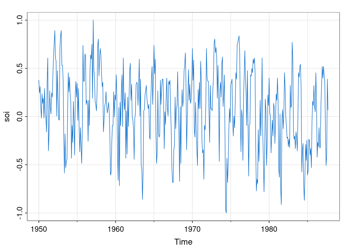
We suppose that a simple random walk model is appropriate for the (hidden) long term trend (so \(\mathsf{G}=1\), and note that the implied VAR(1) model is not stationary), and that the observations are simply noisy observations of that hidden trend (so \(\mathsf{F}=1\)). To complete the model, we suppose that the monthly change in the long term trend has standard deviation 0.01, and that the noise variance associated with the observations has standard deviation 0.5. We can now create the filter and apply it, using the Reduce function and initialising with \(\textbf{m}_0=0\) and \(\mathsf{C}_0=100\).
$m
            [,1]
[1,] -0.03453493

$C
           [,1]
[1,] 0.00495025
This gives us \(\textbf{m}_n\) and \(\mathsf{C}_n\), which might be what we want if we are simply interested in forecasting the future (see next section). However, more likely we want to keep the full set of filtered states and plot them over the data.
fs = Reduce(advance, soi, list(m=0, C=100), acc=TRUE)
fsm = sapply(fs, function(s) s$m)
fsTs = ts(fsm[-1], start=start(soi), freq=frequency(soi))
tsplot(soi, col=4)
lines(fsTs, col=2, lwd=2)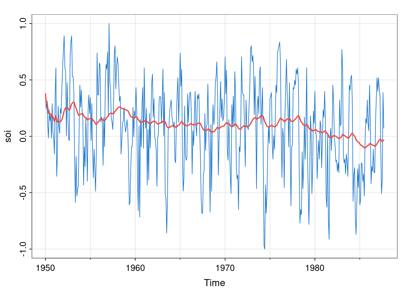
We will look at more interesting DLM models in the next chapter.
7.3 Forecasting
Making forecasts from a DLM is straightforward, since it corresponds to the computation of predictions, and we have already examined this problem in the context of the predict step of a Kalman filter. Suppose that we have a time series of length \(n\), and have run a Kalman filter over the whole data set, culminating in the computation of \(\textbf{m}_n\) and \(\mathsf{C}_n\). We can now define our \(k\)-step ahead forecast distributions as \[\begin{align*} (\mathbf{X}_{n+k}|\mathbf{Y}_{1:n}=\mathbf{y}_{1:n}) &\sim \mathcal{N}(\hat{\mathbf{m}}_n(k), \mathsf{C}_n(k)) \\ (\mathbf{Y}_{n+k}|\mathbf{Y}_{1:n}=\mathbf{y}_{1:n}) &\sim \mathcal{N}(\hat{\mathbf{f}}_n(k), \mathsf{Q}_n(k)), \end{align*}\] for moments \(\hat{\mathbf{m}}_n(k),\ \mathsf{C}_n(k),\ \hat{\mathbf{f}}_n(k),\ \mathsf{Q}_n(k)\) to be determined. Starting from \(\hat{\mathbf{m}}_n(0)=\mathbf{m}_n\) and \(\mathsf{C}_n(0)=\mathsf{C}_n\), we can recursively compute subsequent forecasts for the hidden states via \[ \hat{\mathbf{m}}_n(k) = \mathsf{G}_{n+k}\hat{\mathbf{m}}_n(k-1),\quad \mathsf{C}_n(k) = \mathsf{G}_{n+k}\mathsf{C}_n(k-1)\mathsf{G}_{n+k}^\top+ \mathsf{W}_{n+k}. \] Once we have a forecast for the hidden state, we can compute the moments of the forecast distribution via \[ \hat{\mathbf{f}}_n(k) = \mathsf{F}_{n+k}\hat{\mathbf{m}}_n(k),\quad \mathsf{Q}_n(k) = \mathsf{F}_{n+k}\mathsf{C}_n(k)\mathsf{F}_{n+k}^\top+ \mathsf{V}_{n+k}. \]
7.4 Marginal likelihood
For many applications (including parameter estimation) it is useful to know the marginal likelihood of the data. We can factorise this as \[
L(\mathbf{y}_{1:n}) = \prod_{t=1}^n \pi(\mathbf{y}_t|\mathbf{y}_{1:(t-1)}),
\] but as part of the Kalman filter we compute the component distributions as \[
\pi(\mathbf{y}_t|\mathbf{y}_{1:(t-1)}) = \mathcal{N}(\mathbf{y}_t ; \mathbf{f}_t, \mathsf{Q}_t),
\] so we can compute the marginal likelihood as part of the Kalman filter at little extra cost. In practice we compute the log-likelihood \[
\ell(\mathbf{y}_{1:t}) = \sum_{t=1}^n \log \mathcal{N}(\mathbf{y}_t ; \mathbf{f}_t, \mathsf{Q}_t),
\] We might use a function (such as mvtnorm::dmvnorm) to evaluate the log density of a multivariate normal, but if not, we can write it explicitly in the form \[
\ell(\mathbf{y}_{1:t}) = -\frac{mn}{2}\log 2\pi - \frac{1}{2} \sum_{t=1}^n \left[ \log|\mathsf{Q}_t| + (\mathbf{y}_t-\mathbf{f}_t)^\top\mathsf{Q}_t^{-1}(\mathbf{y}_t-\mathbf{f}_t) \right].
\] Note that this is very straightforward in the case of a univariate time series (scalar \(\mathsf{Q}_t\)), but more generally, there is a good way to evaluate this using the Cholesky decomposition of \(\mathsf{Q}_t\). The details are not important for this course.
7.4.1 Example
We can easily modify our Kalman filter function to compute the marginal likelihood, and apply it to our example problem as follows.
kFilterML = function(G, W, F, V)
  function(mCl, y) {
    m = G %*% mCl$m
    C = (G %*% mCl$C %*% t(G)) + W
    f = F %*% m
    Q = (F %*% C %*% t(F)) + V
    ll = mvtnorm::dmvnorm(y, f, Q, log=TRUE)
    K = t(solve(Q, F %*% C))
    m = m + (K %*% (y - f))
    C = C - (K %*% Q %*% t(K))
    list(m=m, C=C, ll=mCl$ll+ll)
  }

advance = kFilterML(1, 0.01^2, 1, 0.5^2)
Reduce(advance, soi, list(m=0, C=100, ll=0))
$m
[,1]
[1,] -0.03453493
$C
[,1]
[1,] 0.00495025
$ll
[1] -237.29077.5 Smoothing
For the smoothing problem, we want to calculate the marginal at each time given all of the data, \[ \mathbf{X}_t|\mathbf{Y}_{1:n}=\mathbf{y}_{1:n}, \quad t=1,2, \ldots, n. \] We will use a backward recursion to achieve this, known in this context as the Rauch-Tung-Striebel (RTS) smoother. Again, since everything is linear and Gaussian, the marginals will be, so we have \[ (\mathbf{X}_t|\mathbf{Y}_{1:n}=\mathbf{y}_{1:n}) \sim \mathcal{N}(\mathbf{s}_t, \mathsf{S}_t), \] for \(\mathbf{s}_t\), \(\mathsf{S}_t\) to be determined. We know from the forward filter that \(\mathbf{s}_n=\mathbf{m}_n\) and \(\mathsf{S}_n=\mathsf{C}_n\), so we assume that we know \(\mathbf{s}_{t+1}\), \(\mathsf{S}_{t+1}\) for some \(t<n\) and that we want to know \(\mathbf{s}_t\), \(\mathsf{S}_t\).
Since \(\mathbf{X}_{t+1} = \mathsf{G}_{t+1}\mathbf{X}_t + \pmb{\omega}_{t+1}\), we deduce that \[ \left(\left.\begin{array}{c}\mathbf{X}_t\\ \mathbf{X_{t+1}}\end{array}\right|\mathbf{Y}_{1:t}=\mathbf{y}_{1:t}\right) \sim \mathcal{N}\left( \left[\begin{array}{c}\mathbf{m}_t\\ \tilde{\mathbf{m}}_{t+1}\end{array}\right], \left[\begin{array}{cc}\mathsf{C}_t&\mathsf{C}_t\mathsf{G}_{t+1}^\top\\\mathsf{G}_{t+1}\mathsf{C}_t&\tilde{\mathsf{C}}_{t+1}\end{array}\right] \right). \] We can use normal conditioning formula to deduce that \[\begin{multline*} (\mathbf{X}_t|\mathbf{X}_{t+1},\mathbf{Y}_{1:t}=\mathbf{y}_{1:t}) \\ \sim \mathcal{N}\left(\mathbf{m}_t+\mathsf{C}_t\mathsf{G}_{t+1}^\top\tilde{\mathsf{C}}_{t+1}^{-1}[\mathbf{X}_{t+1}-\tilde{\mathbf{m}}_{t+1}], \mathsf{C}_t-\mathsf{C}_t\mathsf{G}_{t+1}^\top\tilde{\mathsf{C}}_{t+1}^{-1}\mathsf{G}_{t+1}\mathsf{C}_t \right). \end{multline*}\] If we define the smoothing gain \(\mathsf{L}_t = \mathsf{C}_t\mathsf{G}_{t+1}^\top\tilde{\mathsf{C}}_{t+1}^{-1}\), then this becomes \[ (\mathbf{X}_t|\mathbf{X}_{t+1},\mathbf{Y}_{1:t}=\mathbf{y}_{1:t}) \sim \mathcal{N}\left(\mathbf{m}_t+\mathsf{L}_t[\mathbf{X}_{t+1}-\tilde{\mathbf{m}}_{t+1}], \mathsf{C}_t-\mathsf{L}_t\tilde{\mathsf{C}}_{t+1}\mathsf{L}_t^\top \right). \] But now, since \(\mathbf{Y}_{(t+1):n}\) is conditionally independent of \(\mathbf{X}_t\) given \(\mathbf{X}_{t+1}\), this distribution is also the distribution of \((\mathbf{X}_t|\mathbf{X}_{t+1},\mathbf{Y}_{1:n}=\mathbf{y}_{1:n})\). So now we can compute \((\mathbf{X}_t|\mathbf{Y}_{1:n}=\mathbf{y}_{1:n})\) by marginalising out \(\mathbf{X}_{t+1}\). First, \[\begin{align*} \mathbf{s}_{t}&= \mathbb{E}[\mathbf{X}_t|\mathbf{Y}_{1:n}=\mathbf{y}_{1:n}]\\ &= \mathbb{E}\left[\mathbb{E}[\mathbf{X}_t|\mathbf{X}_{t+1},\mathbf{Y}_{1:n}=\mathbf{y}_{1:n}]\big|\mathbf{Y}_{1:n}=\mathbf{y}_{1:n}\right]\\ &= \mathbb{E}\left[ \mathbf{m}_t+\mathsf{L}_t[\mathbf{X}_{t+1}-\tilde{\mathbf{m}}_{t+1}] \big|\mathbf{Y}_{1:n}=\mathbf{y}_{1:n}\right]\\ &= \mathbf{m}_t+\mathsf{L}_t[\mathbf{s}_{t+1}-\tilde{\mathbf{m}}_{t+1}] \end{align*}\] Now, \[\begin{align*} \mathsf{S}_t &= \mathbb{V}\mathrm{ar}[\mathbf{X}_t|\mathbf{Y}_{1:n}=\mathbf{y}_{1:n}] \\ &= \mathbb{E}\{\mathbb{V}\mathrm{ar}[\mathbf{X}_t|\mathbf{X}_{t+1},\mathbf{Y}_{1:n}=\mathbf{y}_{1:n}]|\mathbf{Y}_{1:n}=\mathbf{y}_{1:n}\} \\ &\mbox{} \qquad + \mathbb{V}\mathrm{ar}\{\mathbb{E}[\mathbf{X}_t|\mathbf{X}_{t+1},\mathbf{Y}_{1:n}=\mathbf{y}_{1:n}]|\mathbf{Y}_{1:n}=\mathbf{y}_{1:n}\}\\ &= \mathbb{E}\{ \mathsf{C}_t-\mathsf{L}_t\tilde{\mathsf{C}}_{t+1}\mathsf{L}_t^\top|\mathbf{Y}_{1:n}=\mathbf{y}_{1:n} \} \\ &\mbox{} \qquad + \mathbb{V}\mathrm{ar}\{ \mathbf{m}_t+\mathsf{L}_t[\mathbf{X}_{t+1}-\tilde{\mathbf{m}}_{t+1}] |\mathbf{Y}_{1:n}=\mathbf{y}_{1:n} \} \\ &= \mathsf{C}_t-\mathsf{L}_t\tilde{\mathsf{C}}_{t+1}\mathsf{L}_t^\top+ \mathsf{L}_t \mathsf{S}_{t+1} \mathsf{L}_t^\top\\ &= \mathsf{C}_t + \mathsf{L}_t[ \mathsf{S}_{t+1} -\tilde{\mathsf{C}}_{t+1}]\mathsf{L}_t^\top\\ \end{align*}\]
7.5.1 The RTS smoother
To summarise, we receive as input \(\mathbf{s}_{t+1}\) and \(\mathsf{S}_{t+1}\), and compute \[\begin{align*} \mathsf{L}_t &= \mathsf{C}_t\mathsf{G}_{t+1}^\top\tilde{\mathsf{C}}_{t+1}^{-1}\\ \mathbf{s}_t &= \mathbf{m}_t + \mathsf{L}_t[\mathbf{s}_{t+1}-\tilde{\mathbf{m}}_{t+1}] \\ \mathsf{S}_t &= \mathsf{C}_t + \mathsf{L}_t[\mathsf{S}_{t+1}-\tilde{\mathsf{C}}_{t+1}]\mathsf{L}_t^\top, \end{align*}\] re-using computations from the forward Kalman filter as appropriate. Note that the RTS smoother does involve the inversion of a \(p\times p\) matrix.
7.6 Sampling
If we want to understand the joint distribution of the hidden states given the data, generating samples from it will be useful. So, we want to generate exact samples from \[ (\mathbf{X}_{1:n}|\mathbf{Y}_{1:n}=\mathbf{y}_{1:n}). \] Just as for HMMs, it is convenient to do this backwards, starting from the final hidden state. We assume that we have run a Kalman filter forward, but now do sampling on the backward pass. This strategy is known in this context as forward filtering, backward sampling (FFBS). We know that the distribution of the final hidden state is \[ (\mathbf{X}_n|\mathbf{Y}_{1:n}=\mathbf{y}_{1:n}) \sim \mathcal{N}(\mathbf{m}_n, \mathsf{C}_n), \] so we can sample from this to obtain a realisation of \(\mathbf{x}_n\). So now assume that we are given \(\mathbf{x}_{t+1}\) for some \(t<n\), and want to simulate an appropriate \(\mathbf{x}_t\). From the smoothing analysis, we know that \[ (\mathbf{X}_t|\mathbf{X}_{t+1}=\mathbf{x}_{t+1},\mathbf{Y}_{1:n}=\mathbf{y}_{1:n}) \sim \mathcal{N}\left(\mathbf{m}_t+\mathsf{L}_t[\mathbf{x}_{t+1}-\tilde{\mathbf{m}}_{t+1}], \mathsf{C}_t-\mathsf{L}_t\tilde{\mathsf{C}}_{t+1}\mathsf{L}_t^\top \right). \] But since \(\mathbf{X}_t\) is conditionally independent of all future \(\mathbf{X}_s,\ s>t+1\), given \(\mathbf{X}_{t+1}\), this is also the distribution of \((\mathbf{X}_t|\mathbf{X}_{(t+1):n}=\mathbf{x}_{(t+1):n},\mathbf{Y}_{1:n}=\mathbf{y}_{1:n})\) and so we just sample from this, and so on, in a backward pass.
7.7 Parameter estimation
Just as for HMMs, there are a wide variety of Bayesian and likelihood-based approaches to parameter estimation. Here, again, we will keep things simple and illustrate basic numerical optimisation of the marginal log-likelihood of the data.
7.7.1 Example
For our SOI running example, suppose that we are happy with the model structure, but uncertain about the variance parameters \(\mathsf{V}\) and \(\mathsf{W}\). We can do maximum likelihood estimation for those two parameters by first creating a function to evaluate the likelihood for a given parameter combination.
mll = function(wv) {
  advance = kFilterML(1, wv[1], 1, wv[2])
  Reduce(advance, soi, list(m=0, C=100, ll=0))$ll
}

mll(c(0.01^2, 0.5^2))
[1] -237.2907We can see that it reproduces the same log-likelihood as we got before when we evaluate it at our previous guess for \(\mathsf{V}\) and \(\mathsf{W}\). But can we do better than this? Let’s see what optim can do.
$par
[1] 0.05696905 0.03029240

$value
[1] -144.0333

$counts
function gradient
      91       NA

$convergence
[1] 0

$message
NULL
So optim has found parameters with a much higher likelihood, corresponding to a much better fitting model. Note that these optimised parameters apportion the noise more equally between the hidden states and the observation process, and so lead to smoothing the hidden state much less. This may correspond to a better fit, but perhaps not to the fit that we really want. In the context of Bayesian inference, a strong prior on \(\mathsf{V}\) and \(\mathsf{W}\) could help to regularise the problem.
7.8 R package for DLMs
We have seen that it is quite simple to implement the Kalman filter and related computations such as the marginal log-likelihood of the data. However, a very naive implementation such as we have given may not be the most efficient, nor the most numerically stable. Many different approaches to implementing the Kalman filter have been developed over the years, which are mathematically equivalent to the basic Kalman filter recursions, but are more efficient and/or more numerically stable than a naive approach. The dlm R package is an implementation based on the singular value decomposition (SVD), which is significantly more numerically stable than a naive implementation. We will use this package for the study of more interesting DLMs in Chapter 8. More information about this package can be obtained with help(package="dlm") and vignette("dlm", package="dlm"). It is described more fully in Petris, Petrone, and Campagnoli (2009). We can fit our simple DLM to the SOI data as follows.
library(dlm)
mod = dlm(FF=1, GG=1, V=0.5^2, W=0.01^2, m0=0, C0=100)
fs = dlmFilter(soi, mod)
tsplot(soi, col=4, main="Filtered states")
lines(fs$m, col=2, lwd=2)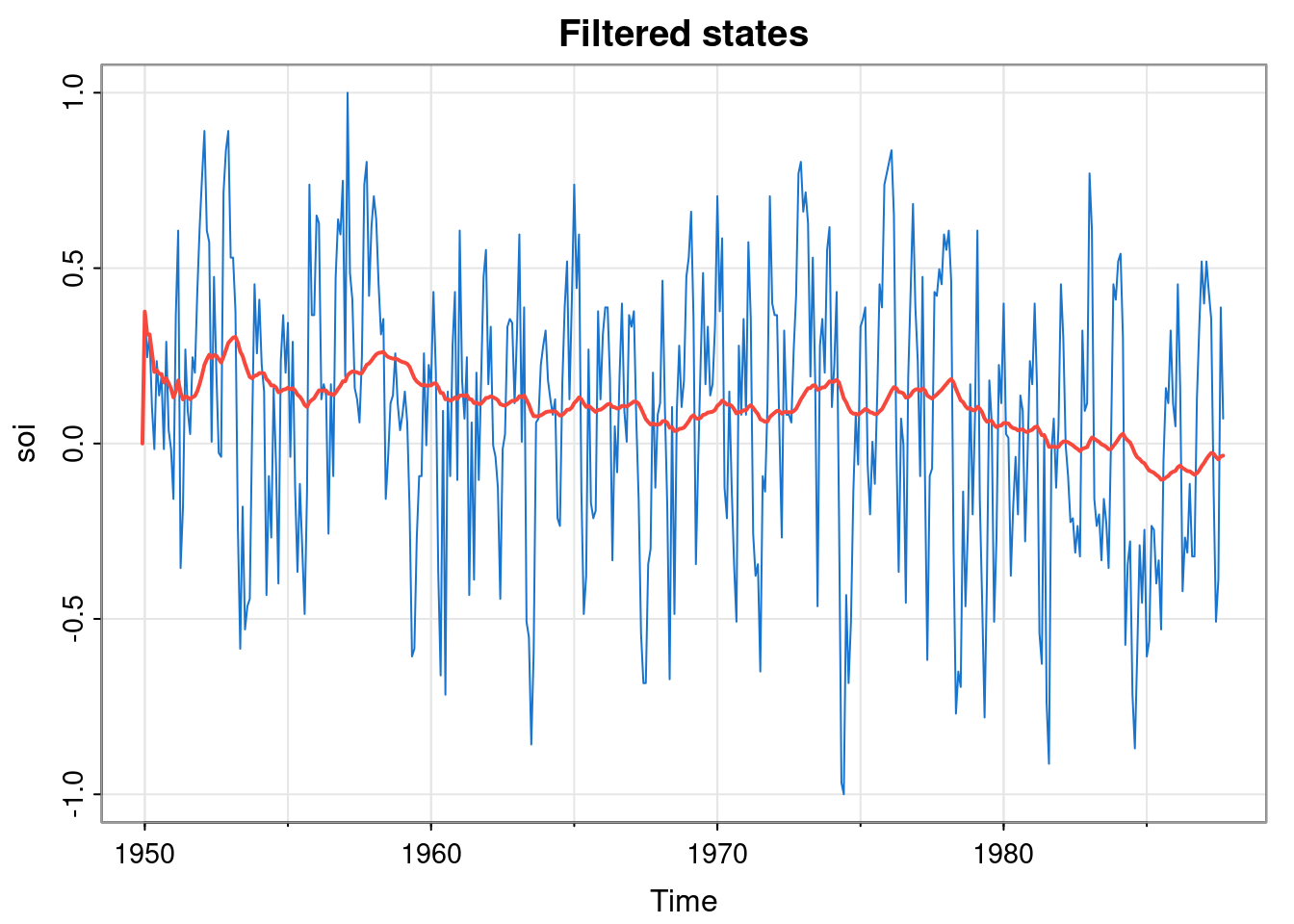
We can also compute the smoothed states.
These are very smooth. We can also optimise the parameters, similar to the approach we have already seen. But note that the dlmMLE optimiser requires that the vector of parameters being optimised is unconstrained, so we use \(\exp\) and \(\log\) to map back and forth between a constrained and unconstrained space.
buildMod = function(lwv)
  dlm(FF=1, GG=1, V=exp(lwv[2]), W=exp(lwv[1]),
    m0=0, C0=100)

opt = dlmMLE(soi, parm=c(log(0.5^2), log(0.01^2)),
  build=buildMod)
opt
$par
[1] -2.865240 -3.496717
$value
[1] -272.2459
$counts
function gradient
35 35
$convergence
[1] 0
$message
[1] "CONVERGENCE: REL_REDUCTION_OF_F <= FACTR*EPSMCH"exp(opt$par)[1] 0.05696943 0.03029668After mapping back to the constrained space, we see that we get the same optimised values as before (the log-likelihood is different, but that is just due to dropping of unimportant constant terms). We can check the smoothed states for this optimised model as follows.
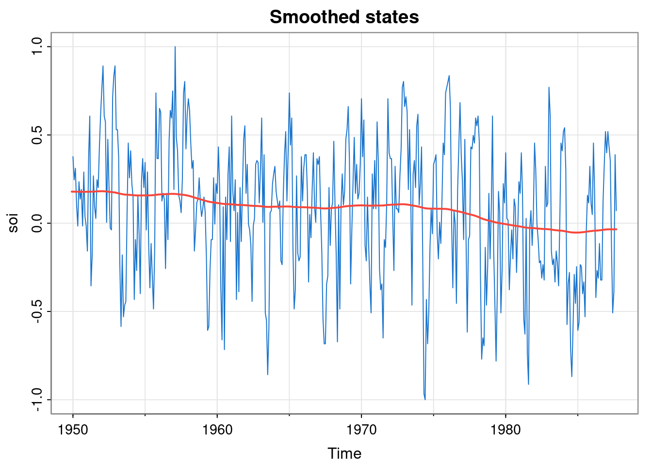
mod = buildMod(opt$par)
ss = dlmSmooth(soi, mod)
tsplot(soi, col=4, main="Smoothed states")
lines(ss$s, col=2, lwd=1.5)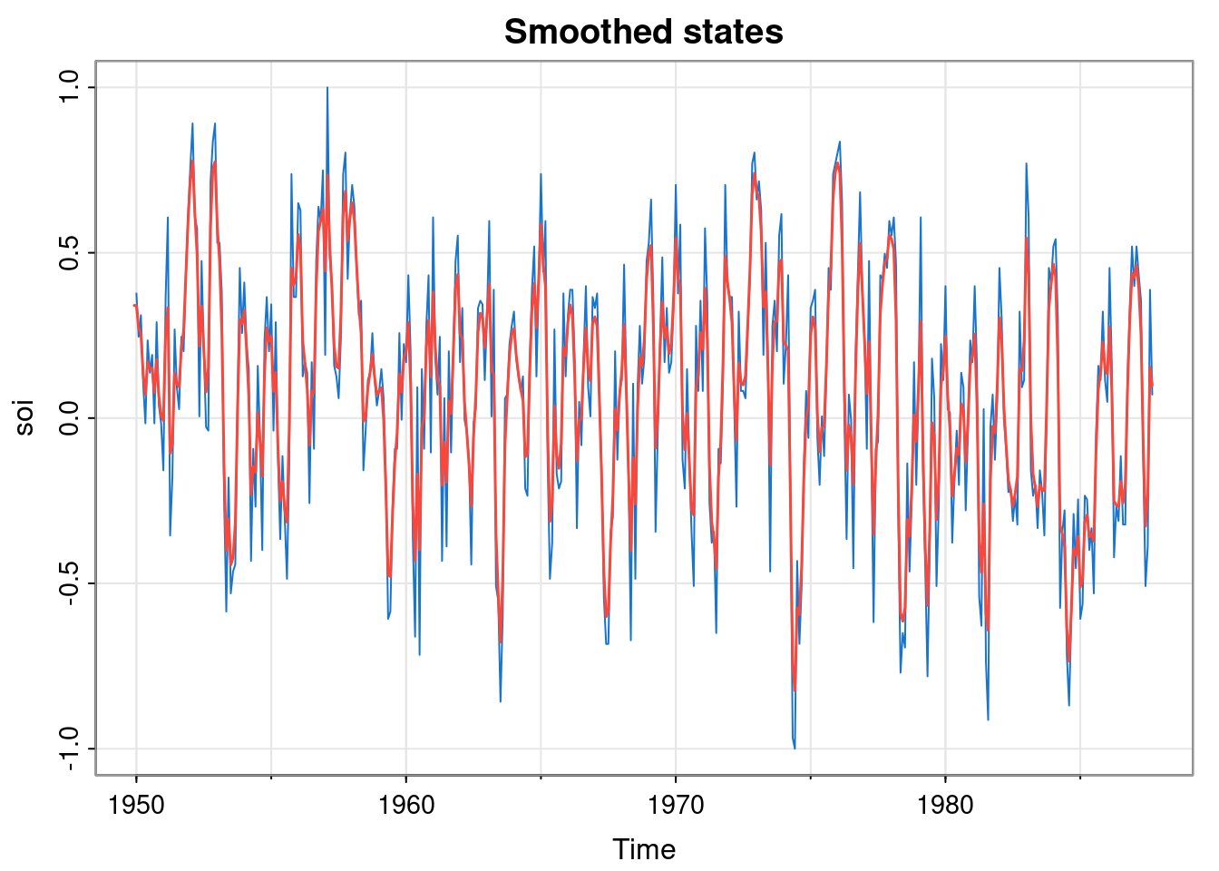
This confirms that the smoothed states for the optimised model are not very smooth. This suggests that our simple random walk model for the data is perhaps not very good.