2  Linear systems

2.1 Introduction

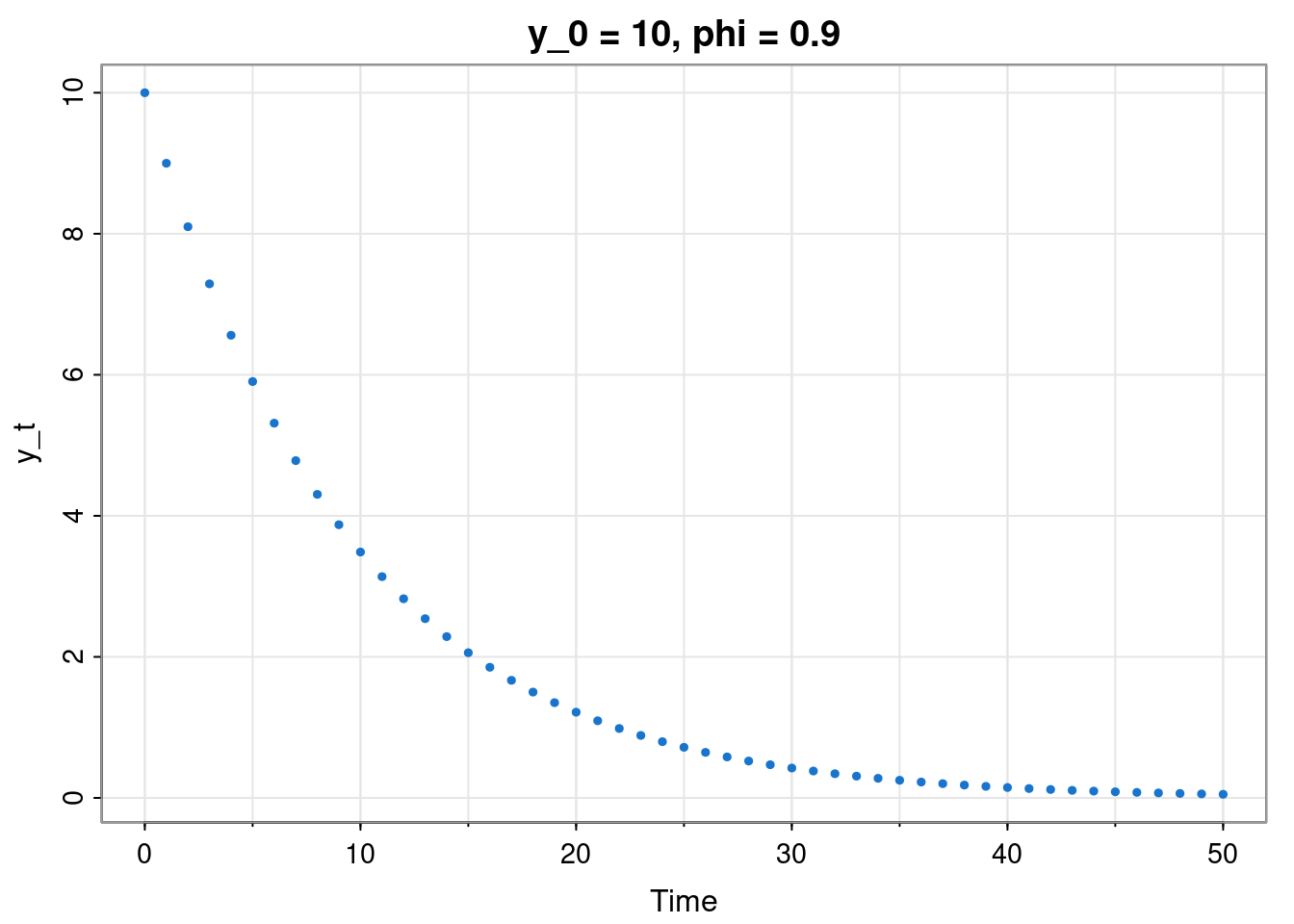
It is likely that you will be familiar with many parts of this chapter, having seen different bits in different courses, in isolation. It might seem a bit strange to look at deterministic linear dynamical systems in a stats course, but it is arguably helpful to see them alongside their stochastic counterparts, in one place, in a consistent notation, to be able to compare and contrast. It could also be argued that this material would belong better in a course on stochastic processes. But time series models are stochastic processes, so we really do need to understand something about stochastic processes to be able to model time series appropriately. This chapter will hopefully make clear how everything links together in a consistent way, and how understanding deterministic dynamical systems helps to understand stochastic counterparts. In particular, it should help to motivate the study of ARMA models in Chapter 3.

2.2 Vector random quantities

Although this course will be mainly concerned with univariate time series, there are many instances in the analysis of time series where vector random quantities and the multivariate normal distribution crop up. It will be useful to recap some essential formulae that you have probably seen before.

2.2.1 Moments

For a random vector \(\mathbf{X}\) with \(i\)th element \(X_i\), the expectation is the vector \(\mathbb{E}[\mathbf{X}]\), of the same length, with \(i\)th element \(\mathbb{E}[X_i]\).

The covariance matrix between vectors \(\mathbf{X}\) and \(\mathbf{Y}\), is the matrix with \((i,j)\)th element \(\mathbb{C}\mathrm{ov}[X_i,Y_j]\), and hence given by \[ \mathbb{C}\mathrm{ov}[\mathbf{X},\mathbf{Y}] = \mathbb{E}\left\{(\mathbf{X}-\mathbb{E}[\mathbf{X}])(\mathbf{Y}-\mathbb{E}[\mathbf{Y}])^\top\right\} = \mathbb{E}[\mathbf{X}\mathbf{Y}^\top] - \mathbb{E}[\mathbf{X}]\mathbb{E}[\mathbf{Y}]^\top. \] It is easy to show that \[ \mathbb{C}\mathrm{ov}[\mathsf{A}\mathbf{X}+\mathbf{b},\mathsf{C}\mathbf{Y}+\mathbf{d}] = \mathsf{A}\mathbb{C}\mathrm{ov}[\mathbf{X},\mathbf{Y}]\mathsf{C}^\top, \] \[ \mathbb{C}\mathrm{ov}[\mathbf{X}+\mathbf{Y},\mathbf{Z}]=\mathbb{C}\mathrm{ov}[\mathbf{X},\mathbf{Z}]+\mathbb{C}\mathrm{ov}[\mathbf{Y},\mathbf{Z}],\quad\text{and}\quad \mathbb{C}\mathrm{ov}[\mathbf{X},\mathbf{Y}]^\top= \mathbb{C}\mathrm{ov}[\mathbf{Y},\mathbf{X}]. \] We define the variance matrix \[ \mathbb{V}\mathrm{ar}[\mathbf{X}] = \mathbb{C}\mathrm{ov}[\mathbf{X},\mathbf{X}], \] from which it follows that \[ \mathbb{V}\mathrm{ar}[\mathsf{A}\mathbf{X}+\mathbf{b}] = \mathsf{A}\mathbb{V}\mathrm{ar}[\mathbf{X}]\mathsf{A}^\top. \]

2.2.2 The multivariate normal distribution

The \(p\)-dimensional multivariate normal distribution can be defined as an affine transformation of a \(p\)-vector of iid standard normal random scalars, and is characterised by its (\(p\)-dimensional) expectation vector, \(\pmb{\mu}\) and (\(p\times p\)) variance matrix, \(\mathsf{\Sigma}\), and written \(\mathcal{N}(\pmb{\mu},\mathsf{\Sigma})\). From this definition it is clear that affine transformations of multivariate normal random quantities will be multivariate normal. It is also relatively easy to deduce that the probability density function (PDF) must take the form \[ \mathcal{N}(\mathbf{x};\pmb{\mu},\mathsf{\Sigma}) = (2\pi)^{-p/2} |\mathsf{\Sigma}|^{-1/2} \exp\left\{-\frac{1}{2}(\mathbf{x}-\pmb{\mu})^\top\mathsf{\Sigma}^{-1}(\mathbf{x}-\pmb{\mu})\right\}. \] From this, relatively routine computations show that if \(\mathbf{X}\) and \(\mathbf{Y}\) are jointly multivariate normal, then both \(\mathbf{X}\) and \(\mathbf{Y}\) are marginally multivariate normal, and further, that the conditional random quantity, \((\mathbf{X}|\mathbf{Y}=\mathbf{y})\) is multivariate normal, and characterised by its conditional mean and variance, \[ \mathbb{E}[\mathbf{X}|\mathbf{Y}=\mathbf{y}] = \mathbb{E}[\mathbf{X}] -\mathbb{C}\mathrm{ov}[\mathbf{X},\mathbf{Y}]\mathbb{V}\mathrm{ar}[\mathbf{Y}]^{-1}(\mathbf{y}-\mathbb{E}[\mathbf{Y}]), \] \[ \mathbb{V}\mathrm{ar}[\mathbf{X}|\mathbf{Y}=\mathbf{y}] = \mathbb{V}\mathrm{ar}[\mathbf{X}] - \mathbb{C}\mathrm{ov}[\mathbf{X},\mathbf{Y}]\mathbb{V}\mathrm{ar}[\mathbf{Y}]^{-1}\mathbb{C}\mathrm{ov}[\mathbf{Y},\mathbf{X}]. \] It is noteworthy that the conditional variance of \(\mathbf{X}\) does not depend on the observed value of \(\mathbf{Y}\) (this is a special property of the multivariate normal distribution).

2.3 First order systems

2.3.1 Deterministic

2.3.1.1 Discrete time

We will start with the simplest linear Markovian model: the linear recurrence relation. We start with the special case \[ y_t = \phi y_{t-1},\quad t\in\{1,2,\ldots\}, \] for some fixed \(\phi\in\mathbb{R}\), initialised with some \(y_0\in\mathbb{R}\). Using substitution we get \(y_1=\phi y_0\), \(y_2=\phi y_1 = \phi^2 y_0\), etc., leading to \[ y_t = \phi^t y_0,\quad t\in\{1,2,\ldots\}. \]

library(astsa)
tsplot(0:50, sapply(0:50, function(t) 10*(0.9)^t),
  type="p", pch=19, cex=0.5, col=4, ylab="y_t",
  main="y_0 = 10, phi = 0.9")

This will be stable for \(|\phi|<1\), leading to \(y_\infty = 0\), and will diverge geometrically for \(|\phi|>1, y_0\not=0\) (other cases require special consideration). Next consider the shifted system \(x_t = y_t + \mu\), so that \[ x_t = \mu + \phi(x_{t-1}-\mu). \] By construction, this system will be stable for \(|\phi|<1\) with \(x_\infty = \mu\). Note that we can re-write this as \[ x_t = \phi x_{t-1} + (1-\phi)\mu, \] so for a system of the form \[ x_t = \phi x_{t-1} + k, \] we know that it will be stable for \(|\phi|<1\) with \(x_\infty = \mu = k/(1-\phi)\). Further, since the general solution in terms of \(\mu\) is \[ x_t = \mu + \phi^t(x_0-\mu) = \phi^t x_0 + (1-\phi^t)\mu , \] the general solution in terms of \(k\) is \[ x_t = \phi^t x_0 + \frac{1-\phi^t}{1-\phi} k. \]

2.3.1.2 Vector discrete time

We can generalise the above system to vectors in the obvious way. Start with \[ \mathbf{y}_t = \mathsf{\Phi} \mathbf{y}_{t-1}, \quad t\in\{1, 2, \ldots\}, \] for some fixed matrix \(\mathsf{\Phi}\in M_{n\times n}\), initialised with vector \(\mathbf{y}_0\in\mathbb{R}^n\). Exactly as above we get \[ \mathbf{y}_t = \mathsf{\Phi}^t \mathbf{y}_0, \] and this will be stable provided that all of the eigenvalues (\(\lambda_i\)) of \(\mathsf{\Phi}\) lie inside the unit circle in the complex plane \((|\lambda_i|<1)\), since then \(\mathsf{\Phi}^t \rightarrow 0\), giving \(\mathbf{y}_\infty = \mathbf{0}\).

Defining \(\mathbf{x}_t = \mathbf{y}_t + \pmb{\mu}\) gives \[ \mathbf{x}_t = \pmb{\mu} + \mathsf{\Phi}(\mathbf{x}_{t-1} - \pmb{\mu}) = \mathsf{\Phi}\mathbf{x}_{t-1} + (\mathbb{I}-\mathsf{\Phi})\pmb{\mu}, \] and so a system of the form \[ \mathbf{x_t} = \mathsf{\Phi}\mathbf{x}_{t-1} + \mathbf{k}, \] in the stable case will have \(\mathbf{x}_\infty = \pmb{\mu} = (\mathbb{I}-\mathsf{\Phi})^{-1}\mathbf{k}\). Note that in the stable case, \(\mathbb{I}-\mathsf{\Phi}\) will be invertible. Further, since the general solution in terms of \(\pmb{\mu}\) is \[ \mathbf{x}_t = \pmb{\mu} + \mathsf{\Phi}^t(\mathbf{x}_0-\pmb{\mu}) = \mathsf{\Phi}^t\pmb{x}_0 + (\mathbb{I}-\mathsf{\Phi}^t)\pmb{\mu} , \] the general solution in terms of \(\mathbf{k}\) is \[ \mathbf{x}_t = \mathsf{\Phi}^t\pmb{x}_0 + (\mathbb{I}-\mathsf{\Phi}^t)(\mathbb{I}-\mathsf{\Phi})^{-1}\mathbf{k}. \]

2.3.1.3 Continuous time

Let’s revert to the scalar case, but switch from discrete time to cts time. The analogous system is the scalar linear ODE \[ \frac{\mathrm{d}y}{\mathrm{d}t} = -\lambda y, \] for some fixed \(\lambda\in\mathbb{R}\), initialised with \(y_0\in\mathbb{R}\). By separating variables (or guessing) we deduce the solution \[ y(t) = y_0 e^{-\lambda t}. \]

tsplot(0:50, sapply(0:50, function(t) 10*exp(-0.1*t)),
  cex=0.5, col=4, ylab="y(t)", main="y_0 = 10, lambda = 0.1")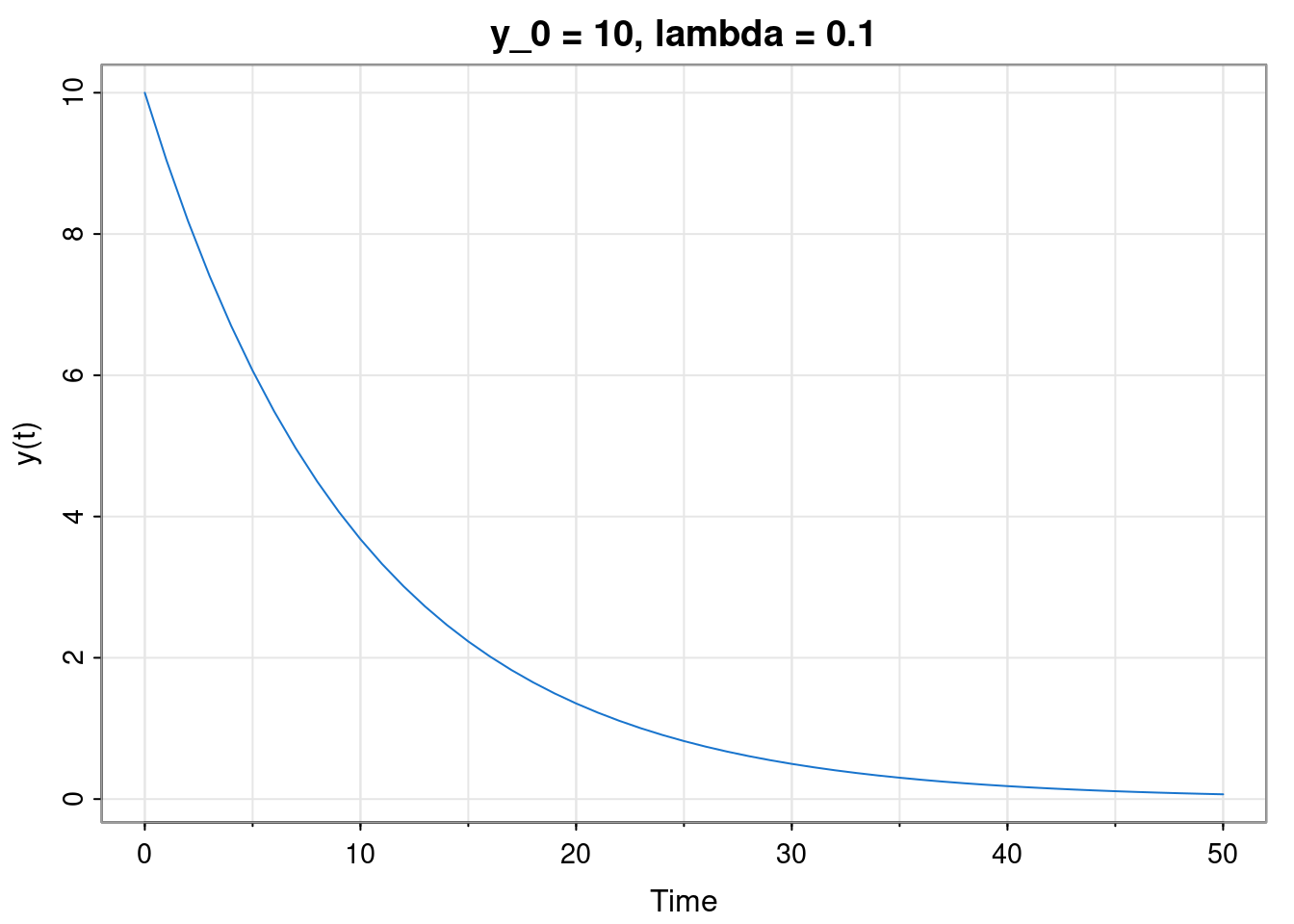

This will be stable for \(\lambda>0\), giving \(y(\infty) = 0\), otherwise likely to diverge (exponentially, but various cases to consider). Note that \(y(t) = \phi^t y_0\) for \(\phi = e^{-\lambda}\), so the continuous time model evaluated at integer times is just a discrete time model.

Defining \(x(t) = y(t) + \mu\) gives \[ \frac{\mathrm{d}x}{\mathrm{d}t} = -\lambda(x-\mu), \] and so for \(\lambda>0\) we will get \(x(\infty) = \mu\). So for a linear ODE of the form \[ \frac{\mathrm{d}x}{\mathrm{d}t} + \lambda x = k, \] we have \(x(\infty) = \mu = k/\lambda\) in the stable case \((\lambda>0)\). Further, since the general solution in terms of \(\mu\) is \[ x(t) = \mu + (x_0-\mu)e^{-\lambda t} = x_0 e^{-\lambda t} + \mu(1-e^{-\lambda t}), \] the general solution in terms of \(k\) is \[ x(t) = x_0 e^{-\lambda t} + \frac{k}{\lambda}(1-e^{-\lambda t}). \]

2.3.1.4 Vector continuous time

The vector equivalent to the previous model is \[ \frac{\mathrm{d}\mathbf{y}}{\mathrm{d}t} = -\mathsf{\Lambda}\mathbf{y}, \] for \(\mathsf{\Lambda}\in M_{n\times n}\), initialised with \(\mathbf{y}_0\in\mathbb{R}^n\). The solution is \[ \mathbf{y}(t) = \exp\{-\mathsf{\Lambda} t\}\mathbf{y}_0, \] where \(\exp\{\cdot\}\) denotes the matrix exponential function. For stability, we need the eigenvalues of \(\exp\{-\mathsf{\Lambda}\}\) to be inside the unit circle. For that we need the real parts of the eigenvalues of \(-\mathsf{\Lambda}\) to be negative. In other words we need the real parts of the eigenvalues of \(\mathsf{\Lambda}\) to be positive. Otherwise the process is likely to diverge, but again, there are various cases to consider. In the stable case we have \(\mathbf{y}(\infty) = \mathbf{0}\).

Note that for integer times, \(t\), we have \(\mathbf{y}(t) = \mathsf{\Phi}^t\mathbf{y}_0\), where \(\mathsf{\Phi} = \exp\{-\mathsf{\Lambda}\}\), so again the solution of the continuous time model at integer times is just a discrete time recurrence relation.

Defining \(\mathbf{x}(t) = \mathbf{y}(t) + \pmb{\mu}\) gives \[ \frac{\mathrm{d}\mathbf{x}}{\mathrm{d}t} = -\mathsf{\Lambda}(\mathbf{x}-\pmb{\mu}), \] with stable limit \(\mathbf{x}(\infty)=\pmb{\mu}\). So, given a linear ODE of the form \[ \frac{\mathrm{d}\mathbf{x}}{\mathrm{d}t} + \mathsf{\Lambda}\mathbf{x} = \mathbf{k}, \] we deduce the stable limit \(\mathbf{x}(\infty)= \pmb{\mu} = \mathsf{\Lambda}^{-1}\mathbf{k}\). Note that in the stable case, \(\mathsf{\Lambda}\) will be invertible. Further, since the general solution in terms of \(\pmb{\mu}\) is \[ \mathbf{x}(t) = \pmb{\mu} + \exp\{-\mathsf{\Lambda} t\}(\mathbf{x}_0-\pmb{\mu}) = \exp\{-\mathsf{\Lambda} t\}\mathbf{x}_0 + (\mathbb{I}-\exp\{-\mathsf{\Lambda} t\})\pmb{\mu}, \] the general solution in terms of \(\mathbf{k}\) is \[ \mathbf{x}(t)= \exp\{-\mathsf{\Lambda} t\}\mathbf{x}_0 + (\mathbb{I}-\exp\{-\mathsf{\Lambda} t\})\mathsf{\Lambda}^{-1}\mathbf{k}. \]

2.3.2 Stochastic

We now turn our attention to the natural linear Gaussian stochastic counterparts of the deterministic systems we have briefly reviewed.

2.3.2.1 Discrete time: AR(1)

We start by looking at a first order Markovian scalar linear Gaussian auto-regressive model, commonly denoted AR(1). The basic form of the model can be written \[ Y_t = \phi Y_{t-1} + \varepsilon_t, \quad \varepsilon_t\sim \mathcal{N}(0,\sigma^2), \tag{2.1}\] for some fixed \(\phi\in\mathbb{R}\), noise variance \(\sigma>0\), and for now we will assume that it is initialised at some fixed \(Y_0 = y_0\in\mathbb{R}\). It is just a linear recurrence relation with some iid Gaussian noise added at each time step. It’s also an appropriate auto-regressive linear filter applied to iid noise.

tsplot(filter(rnorm(80, 0, 0.5), 0.9, "rec", init=10),
  type="p", col=4, pch=19, cex=0.5, ylab="Y_t",
  main="y_0=10, alpha=0.9, sigma=0.5")
abline(h=0, col=3, lwd=2)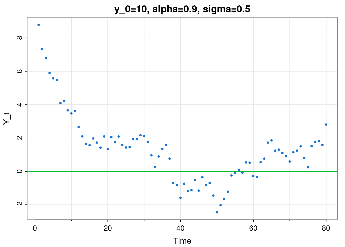

Taking the expectation of Equation 2.1 gives \[ \mathbb{E}[Y_t] = \phi\mathbb{E}[Y_{t-1}] \] In other words, the expectation satisfies a linear recurrence relation with solution \[ \mathbb{E}[Y_t] = \phi^t y_0. \] In the stable case (\(|\phi|<1\)) we will have limiting expectation 0. But this is a random process, so just knowing about its expectation isn’t enough. Next take the variance of Equation 2.1 \[ \mathbb{V}\mathrm{ar}[Y_t] = \phi^2\mathbb{V}\mathrm{ar}[Y_{t-1}] + \sigma^2, \] and note that the variance also satisfies a linear recurrence relation with solution \[ \mathbb{V}\mathrm{ar}[Y_t] = \frac{1-\phi^{2t}}{1-\phi^2}\sigma^2, \] since we are assuming here that \(\mathbb{V}\mathrm{ar}[Y_0]=0\). So, since each update is a linear transformation of a Gaussian random variable, we know that the marginal distribution at each time must be Gaussian, and hence \[ Y_t \sim \mathcal{N}\left(\phi^t y_0, \frac{1-\phi^{2t}}{1-\phi^2}\sigma^2 \right). \] The limiting distribution (in the stable case, \(|\phi|<1\)) is therefore \[ Y_\infty \sim \mathcal{N}\left(0, \frac{\sigma^2}{1-\phi^2} \right). \] So, in the case of a stochastic model, stability implies that the process converges to some limiting probability distribution, and not some fixed point. But the moments of that distribution (such as the mean and variance), are converging to a fixed point.

If we now consider the shifted system \(X_t = Y_t + \mu\), for some fixed \(\mu\in\mathbb{R}\), we have \[ X_t = \mu + \phi(X_{t-1}-\mu) + \varepsilon_t = \phi X_{t-1} + (1-\phi)\mu + \varepsilon_t. \] Now, \(\mathbb{V}\mathrm{ar}[X_t]=\mathbb{V}\mathrm{ar}[Y_t]\), but \[ \mathbb{E}[X_t] = \mathbb{E}[Y_t]+\mu = \phi^t y_0 + \mu = \phi^t(x_0-\mu) + \mu = \phi^t x_0 + (1-\phi^t)\mu, \] so \[ X_t \sim \mathcal{N}\left( \phi^t x_0 + (1-\phi^t)\mu, \frac{1-\phi^{2t}}{1-\phi^2}\sigma^2 \right). \] Consequently, if presented with an auto-regression in the form \[ X_t = \phi X_{t-1} + k + \varepsilon_t, \] for some fixed \(k\in\mathbb{R}\), just put \(k=(1-\phi)\mu\) to get \[ X_t \sim \mathcal{N}\left( \phi^t x_0 + \frac{1-\phi^t}{1-\phi} k, \frac{1-\phi^{2t}}{1-\phi^2}\sigma^2 \right), \] which obviously has limiting distribution \[ X_\infty \sim \mathcal{N}\left(\frac{k}{1-\phi}, \frac{\sigma^2}{1-\phi^2}\right). \]

2.3.2.1.1 Stationarity and further properties

Let’s go back to the centred process \(Y_t\) (to keep the algebra a bit simpler) and think more carefully about what we have been doing. Everything was conditioned on the initial value of the process, \(Y_0=y_0\), so when we deduced the “marginal” distribution for \(Y_t\), this should more correctly have been considered to be the conditional distribution of \(Y_t\) given \(Y_0=y_0\), \[ (Y_t|Y_0=y_0) \sim \mathcal{N}\left(\phi^t y_0, \frac{1-\phi^{2t}}{1-\phi^2}\sigma^2 \right). \] This conditional distribution can be thought of as a transition kernel of the stochastic process. Being clear about this then allows us to consider other initialisation strategies, including random initialisation. In particular, suppose now that \(Y_0\) is drawn from a normal distribution (independent of the process), \(Y_0 \sim \mathcal{N}(\mu_0, \sigma_0^2)\). Since \(Y_0\) is normal and \(Y_t|Y_0\) is normal with linear dependence on \(Y_0\), then \(Y_0\) and \(Y_t\) are jointly normal, and so is the (true) marginal for \(Y_t\). The mean of this marginal can be computed with the law of total expectation, \[ \mathbb{E}[Y_t] = \mathbb{E}(\mathbb{E}[Y_t|Y_0]) = \mathbb{E}(\phi^t Y_0) = \phi^t\mathbb{E}(Y_0)=\phi^t\mu_0. \] Similarly, the variance can be computed with the law of total variance, \[\begin{align*} \mathbb{V}\mathrm{ar}[Y_t] &= \mathbb{E}(\mathbb{V}\mathrm{ar}[Y_t|Y_0]) + \mathbb{V}\mathrm{ar}(\mathbb{E}[Y_t|Y_0]) \\ &= \mathbb{E}\left( \frac{1-\phi^{2t}}{1-\phi^2}\sigma^2\right) + \mathbb{V}\mathrm{ar}(\phi^t Y_0)\\ &= \frac{1-\phi^{2t}}{1-\phi^2}\sigma^2 + \phi^{2t}\sigma_0^2 \end{align*}\] Consequently, the marginal distribution is \[ Y_t \sim \mathcal{N}\left( \phi^t\mu_0 , \frac{1-\phi^{2t}}{1-\phi^2}\sigma^2 + \phi^{2t}\sigma_0^2 \right). \] What happens if we choose the limiting distribution as the initial distribution? ie. if we choose \(\mu_0=0\) and \(\sigma_0^2 = \sigma^2/(1-\phi^2)\)? Subbing these in to the above and simplifying gives \[ Y_t \sim \mathcal{N}\left( 0 , \frac{\sigma^2}{1-\phi^2}\right). \] So, the limiting distribution is stationary in the sense that if the process is initialised with this distribution, it will keep exactly this marginal distribution for all future times. In this case, since the dynamics of the process do not depend explicitly on time and the marginal distribution is the same at each time, it is clear that the full joint distribution of the process is invariant under a time shift. There are various short-cuts one can deploy to deduce the properties of such stationary stochastic processes.

The covariance \(\mathbb{C}\mathrm{ov}(Y_s, Y_{s+t}), \ t\geq 0\) will only depend on the value of \(t\), and will be independent of the value of \(s\). We can call this the auto-covariance function, \(\gamma_t = \mathbb{C}\mathrm{ov}(Y_s, Y_{s+t})\). This can be exploited in order to deduce properties of the process. eg. if we start with the dynamics \[ Y_s = \phi Y_{s-1} + \varepsilon_s, \] multiply by \(Y_{s-t}\), \[ Y_{s-t}Y_s = \phi Y_{s-t}Y_{s-1} + Y_{s-t}\varepsilon_s , \] and take expectations \[ \mathbb{E}[Y_{s-t}Y_s] = \phi \mathbb{E}[Y_{s-t}Y_{s-1}] + \mathbb{E}[Y_{s-t}\varepsilon_s]. \] For \(t>0\) the final expectation is 0, leading to the recurrence \[ \gamma_t = \phi \gamma_{t-1}, \] with solution \[ \gamma_t = \gamma_0 \phi^t = \frac{\phi^t \sigma^2}{1-\phi^2}. \] The corresponding auto-correlation function, \(\rho_t = \mathbb{C}\mathrm{orr}(Y_s, Y_{s+t}) = \gamma_t/\gamma_0\) is \[ \rho_t = \phi^t. \] So, the AR(1) process, in the stable case, admits a stationary distribution, but is not iid, having correlations that die away geometrically as values become further apart in time.

2.3.2.2 Vector discrete time: VAR(1)

The obvious multivariate generalisation of the AR(1) process is the first-order vector auto-regressive process, denoted VAR(1): \[ \mathbf{Y}_t = \mathsf{\Phi} \mathbf{Y}_{t-1} + \pmb{\varepsilon}_t, \quad \pmb{\varepsilon}_t \sim \mathcal{N}(0, \mathsf{\Sigma}), \tag{2.2}\] for some fixed \(\mathsf{\Phi}\in M_{n\times n}\), \(\mathsf{\Sigma}\) an \(n\times n\) symmetric positive semi-definite (PSD) variance matrix, and again assuming a given fixed initial condition \(\mathbf{Y}_0 = \mathbf{y_0}\in\mathbb{R}^n\).

Taking the expectation of Equation 2.2 we get \[ \mathbb{E}[\mathbf{Y}_t] = \mathsf{\Phi}\mathbb{E}[\mathbf{Y}_{t-1}], \] which is a linear recurrence with solution \[ \mathbb{E}[\mathbf{Y}_t] = \mathsf{\Phi}^t \mathbf{y}_0. \] In the stable case (eigenvalues of \(\mathsf{\Phi}\) inside the unit circle), this will have a limit of \(\mathbf{0}\). If we now take the variance of Equation 2.2 we get \[ \mathbb{V}\mathrm{ar}[\mathbf{Y}_t] = \mathsf{\Phi} \mathbb{V}\mathrm{ar}[\mathbf{Y}_{t-1}] \mathsf{\Phi}^\top+ \mathsf{\Sigma}. \] This is actually a kind of linear recurrence for matrices, but it’s more complicated than the examples we considered earlier. However, if we let \(\mathsf{V}\) be the solution of the discrete Lyapunov equation \[ \mathsf{V} = \mathsf{\Phi} \mathsf{V} \mathsf{\Phi}^\top+ \mathsf{\Sigma}, \] we can check by direct substitution that \[ \mathbb{V}\mathrm{ar}[\mathbf{Y}_t] = \mathsf{V} - \mathsf{\Phi}^t\mathsf{V}{\mathsf{\Phi}^t}^\top \] solves the recurrence relation. There are standard direct methods for solving Lyapunov equations (eg. netcontrol::dlyap). It is then clear that in the stable case the limiting variance is \(\mathsf{V}\). Since updates are linear transformations of multivariate normals, every marginal is normal, and so we have \[ \mathbf{Y}_t \sim \mathcal{N}\left(\mathsf{\Phi}^t \mathbf{y}_0, \mathsf{V} - \mathsf{\Phi}^t\mathsf{V}{\mathsf{\Phi}^t}^\top\right), \] with limit \[ \mathbf{Y}_\infty \sim \mathcal{N}(\mathbf{0}, \mathsf{V}). \] If we now consider the shifted system \(\mathbf{X}_t = \mathbf{Y}_t + \pmb{\mu}\), we have \(\mathbb{E}[\mathbf{X}_t] = \mathsf{\Phi}^t\mathbf{x_0} + (\mathbb{I}-\mathsf{\Phi}^t)\pmb{\mu}\) and \(\mathbb{V}\mathrm{ar}[\mathbf{X}_t]=\mathbb{V}\mathrm{ar}[\mathbf{Y}_t]\) following very similar arguments to those we have already seen, and so \[ \mathbf{X}_t \sim \mathcal{N}\left( \mathsf{\Phi}^t\mathbf{x_0} + (\mathbb{I}-\mathsf{\Phi}^t)\pmb{\mu}, \mathsf{V} - \mathsf{\Phi}^t\mathsf{V}{\mathsf{\Phi}^t}^\top\right). \] Consequently, if presented with an auto-regressive model in the form \[ \mathbf{X}_t = \mathsf{\Phi}\mathbf{X}_{t-1} + \mathbf{k} + \pmb{\varepsilon}_t, \] just put \(\mathbf{k}=(\mathbb{I}-\mathsf{\Phi})\pmb{\mu}\) to get \[ \mathbf{X}_t \sim \mathcal{N}\left( \mathsf{\Phi}^t\mathbf{x_0} + (\mathbb{I}-\mathsf{\Phi}^t)(\mathbb{I}-\mathsf{\Phi})^{-1}\mathbf{k}, \mathsf{V} - \mathsf{\Phi}^t\mathsf{V}{\mathsf{\Phi}^t}^\top\right), \] with limit \[ \mathbf{X}_\infty \sim \mathcal{N}\left((\mathbb{I}-\mathsf{\Phi})^{-1}\mathbf{k}, \mathsf{V}\right). \]

2.3.2.2.1 Stationarity and further properties

As for the scalar case, what we have deduced above is actually the transition kernel of the process conditional on an initial condition \(\mathbf{Y}_0=\mathbf{y}_0\). We can check that in the stable case if we initialise the process with the limiting distribution it is stationary. So again, in the stable case we can consider the stationary process implied by these dynamics, and use stationarity in order to deduce properties of the process.

Here we will look at the covariance function \(\mathsf{\Gamma}_t=\mathbb{C}\mathrm{ov}(\mathbf{Y}_s, \mathbf{Y}_{s+t})\) (noting that \(\mathsf{\Gamma}_{-t}=\mathsf{\Gamma}_t^\top\)) using a similar approach as before. \[\begin{align*} \mathbf{Y}_s &= \mathsf{\Phi}\mathbf{Y}_{s-1} + \pmb{\varepsilon}_s \\ \Rightarrow \mathbf{Y}_s \mathbf{Y}_{s-t}^\top&= \mathsf{\Phi}\mathbf{Y}_{s-1} \mathbf{Y}_{s-t}^\top+ \pmb{\varepsilon}_s \mathbf{Y}_{s-t}^\top\\ \Rightarrow \mathbb{E}[\mathbf{Y}_s \mathbf{Y}_{s-t}^\top] &= \mathsf{\Phi}\mathbb{E}[\mathbf{Y}_{s-1} \mathbf{Y}_{s-t}^\top] + \mathbb{E}[\pmb{\varepsilon}_s \mathbf{Y}_{s-t}^\top] \\ \Rightarrow \mathsf{\Gamma}_{-t} &= \mathsf{\Phi}\mathsf{\Gamma}_{1-t} \quad\text{for $t>0$} \\ \Rightarrow \mathsf{\Gamma}_{t}^\top&= \mathsf{\Phi}\mathsf{\Gamma}_{t-1}^\top\\ \Rightarrow \mathsf{\Gamma}_{t} &= \mathsf{\Gamma}_{t-1}\mathsf{\Phi}^\top\\ \Rightarrow \mathsf{\Gamma}_{t} &= \mathsf{\Gamma}_{0}{\mathsf{\Phi}^t}^\top\\ \Rightarrow \mathsf{\Gamma}_{t} &= \mathsf{V}{\mathsf{\Phi}^t}^\top\\ \end{align*}\]

2.3.2.3 Continuous time: OU

Switching back to the scalar case but moving to cts time we must describe our linear Markov process using a stochastic differential equation (SDE), \[ \mathrm{d}Y(t) = -\lambda Y(t)\,\mathrm{d}t + \sigma\,\mathrm{d}W(t),\quad Y(0)=y_0, \tag{2.3}\] for fixed \(\lambda, \sigma>0\), known as the Ornstein–Uhlenbeck (OU) process. Here, \(\mathrm{d}W(t)\) should be interpreted as increments of a Wiener process (often referred to as Brownian motion), and hence, informally, \(\mathrm{d}W(t)\sim \mathcal{N}(0,\mathrm{d}t)\). We are going to be very informal in our treatment of SDEs - they are a little bit tangential to the main thrust of the course, and careful treatment gets very technical very quickly. It is helpful to write Equation 2.3 in the form \[\begin{align*} Y(t+\mathrm{d}t) &= Y(t)-\lambda Y(t)\,\mathrm{d}t + \sigma\,\mathrm{d}W(t) \\ &= (1-\lambda\,\mathrm{d}t)Y(t) + \sigma\,\mathrm{d}W(t), \end{align*}\] so then taking expectations gives \[ \mathbb{E}[Y(t+\mathrm{d}t)] = (1-\lambda\,\mathrm{d}t)\mathbb{E}[Y(t)]. \]

T=50; dt=0.1; lambda=0.2; sigma=0.5; y0=10
times = seq(0, T, dt)
y = filter(rnorm(length(times), 0, sigma*sqrt(dt)), 
      1 - lambda*dt, "rec", init=y0)
tsplot(times, y, col=4, ylab="Y(t)", 
  main=paste("lambda =",lambda,"sigma =",sigma,"y0 =",y0))
abline(h=0, col=3, lwd=2)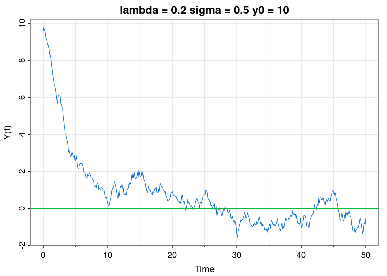

Defining \(m(t) = \mathbb{E}[Y(t)]\) leads to \[ m(t+\mathrm{d}t) = (1-\lambda\,\mathrm{d}t)m(t), \] and re-arranging gives \[ \frac{m(t+\mathrm{d}t)-m(t)}{\mathrm{d}t} = -\lambda\, m(t). \] In other words, \[ \frac{\mathrm{d}m}{\mathrm{d}t} = -\lambda m. \] So as you might have guessed, the expectation satisfies the obvious simple linear ODE, with solution \[ m(t) = \mathbb{E}[Y(t)] = y_0 e^{-\lambda t}. \] Now instead if we evaluate the variance we get \[\begin{align*} \mathbb{V}\mathrm{ar}[Y(t+\mathrm{d}t)] &= (1-\lambda\,\mathrm{d}t)^2\mathbb{V}\mathrm{ar}[Y(t)] + \sigma^2\,\mathrm{d}t \\ &= (1-2\lambda\,\mathrm{d}t)\mathbb{V}\mathrm{ar}[Y(t)] + \sigma^2\,\mathrm{d}t, \end{align*}\] since \(\mathrm{d}t^2\simeq 0\). Again, things might be clearer if we define \(v(t) = \mathbb{V}\mathrm{ar}[Y(t)]\) to get \[ v(t+\mathrm{d}t) = (1-2\lambda\,\mathrm{d}t)v(t) + \sigma^2\,\mathrm{d}t, \] and re-arranging gives \[ \frac{v(t+\mathrm{d}t)-v(t)}{\mathrm{d}t} = -2\lambda\,v(t) + \sigma^2. \] In other words \[ \frac{\mathrm{d}v}{\mathrm{d}t} = -2\lambda\,v + \sigma^2. \] So the variance also satisfies a simple linear ODE, with solution \[ v(t) = \frac{\sigma^2}{2\lambda}(1-e^{-2\lambda t}). \] Again, since everything is linear Gaussian, so will be the solution, so \[ Y(t) \sim \mathcal{N}\left( e^{-\lambda t} y_0, \frac{\sigma^2}{2\lambda}(1-e^{-2\lambda t}) \right), \] with limit \[ Y(\infty) \sim \mathcal{N}(0, \sigma^2/(2\lambda)). \] It should be noted that when considered at integer times, this process is exactly an AR(1) with \(\phi=e^{-\lambda}\), though the role of the parameter \(\sigma\) in the two models is slightly different.

Again, we can consider the shifted system, \(X(t) = Y(t) + \mu\). We get \(\mathbb{E}[X(t)] = e^{-\lambda t}x_0 + (1-e^{-\lambda_t})\mu\), \(\mathbb{V}\mathrm{ar}[X(t)]=\mathbb{V}\mathrm{ar}[Y(t)]\), so \[ X(t) \sim \mathcal{N}\left( e^{-\lambda t} x_0 + (1-e^{-\lambda t})\mu, \frac{\sigma^2}{2\lambda}(1-e^{-2\lambda t}) \right) \] for the SDE \[ \mathrm{d}X(t) = -\lambda[X(t)-\mu]\,\mathrm{d}t + \sigma\,\mathrm{d}W(t). \]

2.3.2.3.1 Stationarity and further properties

Again, what we have considered above is really the transition kernel of the continuous time process. But in the stable case, we get a limiting distribution, and we can easily check that this limiting distribution is stationary. So in the stable case, the OU model determines a stationary stochastic process in continuous time. Since everything is Gaussian, it is a one-dimensional stationary Gaussian process (GP). In fact, it turns out to be the only stationary GP with the (first-order) Markov property. We know its mean and variance, so to fully characterise the process we just need to know its auto-covariance or auto-correlation function. We can calculate this analogously to the discrete time case. Start by considering the dynamics of the process at time \(s\). \[\begin{align*} Y(s+\mathrm{d}t) &= (1-\lambda\,\mathrm{d}t)Y(s) + \sigma\, \mathrm{d}W(s) \\ \Rightarrow Y(s-t)Y(s+\mathrm{d}t) &= (1-\lambda\,\mathrm{d}t)Y(s-t)Y(s) + \sigma Y(s-t)\, \mathrm{d}W(s) \\ \Rightarrow \gamma(t+st) &= (1-\lambda\,\mathrm{d}t)\gamma(t)\quad \text{for $t>0$} \\ \Rightarrow \frac{\mathrm{d}\gamma}{\mathrm{d}t} &= -\lambda \gamma \\ \Rightarrow \gamma(t) &= \gamma(0) e^{-\lambda t} \end{align*}\] So \(\rho(t) = e^{-\lambda t}, \forall t>0\). Since \(\rho(t)=\rho(-t)\) for scalar stationary processes, in general we have \[ \rho(t) = e^{-\lambda |t|}, \] and this correlation function completes the characterisation of an OU process as a GP.

2.3.2.4 Vector continuous time: VOU

We can now consider the obvious multivariate generalisation of the OU process, the vector OU (VOU) process, \[ \mathrm{d}\mathbf{Y}(t) = -\mathsf{\Lambda}\mathbf{Y}(t)\,\mathrm{d}t + \mathsf{\Omega}\,\mathrm{d}\mathbf{W}(t),\quad \mathbf{Y}(0)=\mathbf{y}_0, \] where now fixed \(\mathsf{\Lambda}, \mathsf{\Omega}\in M_{n\times n}\) and \(\mathrm{d}\mathbf{W}(t)\) represents increments of a vector Wiener process, informally \(\mathrm{d}\mathbf{W}(t)\sim \mathcal{N}(\mathbf{0},\mathbb{I}\mathrm{d}t)\). Again, it is helpful to re-write the SDE, informally, as \[ \mathbf{Y}(t+\mathrm{d}t) = (\mathbb{I}-\mathsf{\Lambda}\,\mathrm{d}t)\mathbf{Y}(t) + \mathsf{\Omega}\,\mathrm{d}\mathbf{W}(t). \] Taking expectations and defining \(\mathbf{m}(t)=\mathbb{E}[\mathbf{Y}(t)]\) leads, unsurprisingly, to the ODE \[ \frac{\mathrm{d}\mathbf{m}}{\mathrm{d}t} = -\mathsf{\Lambda} \mathbf{m}, \] with solution \[ \mathbf{m}(t) = \mathbb{E}[\mathbf{Y}(t)] = \exp\{-\mathsf{\Lambda} t\}\mathbf{y}_0. \] Stability of the fixed point of \(\mathbf{0}\) will require the real parts of the eigenvalues of \(\mathsf{\Lambda}\) to be positive.

Taking the variance gives \[ \mathbb{V}\mathrm{ar}[\mathbf{Y}(t+\mathrm{d}t)] = (\mathbb{I}-\mathsf{\Lambda}\,\mathrm{d}t)\mathbb{V}\mathrm{ar}[\mathbf{Y}(t)](\mathbb{I}-\mathsf{\Lambda}\,\mathrm{d}t)^\top+ \mathsf{\Omega}\mathsf{\Omega}^\top\mathrm{d}t. \] Putting \(\mathsf{V}(t) = \mathbb{V}\mathrm{ar}[\mathbf{Y}(t)]\) and \(\mathsf{\Sigma} = \mathsf{\Omega}\mathsf{\Omega}^\top\) leads to the linear matrix ODE \[ \frac{\mathrm{d}\mathsf{V}}{\mathrm{d}t} = -\mathsf{\Lambda} \mathsf{V} - \mathsf{V}\mathsf{\Lambda}^\top+ \mathsf{\Sigma}. \] Even without explicitly solving, it is clear that at the fixed point we will have the continuous Lyapunov equation \[ \mathsf{\Lambda} \mathsf{V}_\infty + \mathsf{V}_\infty \mathsf{\Lambda}^\top= \mathsf{\Sigma}. \] Again, there are standard direct methods for solving this for \(\mathsf{V}_\infty\) (eg. maotai::lyapunov). Analogously with the discrete time case, we can verify by direct substitution that the solution to the variance ODE is given by \[ \mathsf{V}(t) = \mathsf{V}_\infty - \exp\{-\mathsf{\Lambda} t\}\mathsf{V}_\infty\exp\{-\mathsf{\Lambda} t\}^\top. \] Everything is linear and multivariate normal, so the marginal is too, giving \[ \mathbf{Y}(t) \sim \mathcal{N}\left( \exp\{-\mathsf{\Lambda} t\}\mathbf{y}_0\, , \mathsf{V}_\infty - \exp\{-\mathsf{\Lambda} t\}\mathsf{V}_\infty\exp\{-\mathsf{\Lambda} t\}^\top\right), \] with limiting distribution \[ \mathbf{Y(\infty)} \sim \mathcal{N}(\mathbf{0}, \mathsf{V}_\infty) \] in the stable case. We can analyse the shifted system \(\mathbf{X}(t)=\mathbf{Y}(t)+\pmb{\mu}\) as we have seen previously to obtain \[ \mathbf{X}(t) \sim \mathcal{N}\left( \exp\{-\mathsf{\Lambda} t\}\mathbf{y}_0 + (\mathbb{I}-\exp\{-\mathsf{\Lambda} t\})\pmb{\mu}\, , \mathsf{V}_\infty - \exp\{-\mathsf{\Lambda} t\}\mathsf{V}_\infty\exp\{-\mathsf{\Lambda} t\}^\top\right) \] as the marginal for the SDE \[ \mathrm{d}\mathbf{X}(t) = -\mathsf{\Lambda}[\mathbf{X}(t)-\pmb{\mu}]\mathrm{d}t + \mathsf{\Omega}\,\mathrm{d}\mathbf{W}(t). \]

2.3.2.4.1 Stationarity and further properties

Again, we have so far characterised the transition kernel of the VOU process. But in the stable case, we can again check that the limiting distribution is stationary, and so the stable VOU process admits a stationary solution. This stationary solution is a vector-valued one-dimensional GP, and since we know its mean and variance, we just need the auto-covariance function to complete its GP characterisation. Again, we start with the dynamics at time \(s\). \[\begin{align*} \mathbf{Y}(s+\mathrm{d}t) &= (\mathbb{I}-\mathsf{\Lambda}\,\mathrm{d}t)\mathbf{Y}(s) + \mathsf{\Omega}\,\mathrm{d}\mathbf{W}(s) \\ \Rightarrow \mathbf{Y}(s+\mathrm{d}t)\mathbf{Y}(s-t)^\top&= (\mathbb{I}-\mathsf{\Lambda}\,\mathrm{d}t)\mathbf{Y}(s)\mathbf{Y}(s-t)^\top+ \mathsf{\Omega}\,\mathrm{d}\mathbf{W}(s)\mathbf{Y}(s-t)^\top\\ \Rightarrow \mathsf{\Gamma}(-t-\mathrm{d}t) &= (\mathbb{I}-\mathsf{\Lambda}\,\mathrm{d}t)\mathsf{\Gamma}(-t),\quad \text{for $t>0$} \\ \Rightarrow \mathsf{\Gamma}(t+\mathrm{d}t)^\top&= (\mathbb{I}- \mathsf{\Lambda}\,\mathrm{d}t)\mathsf{\Gamma}(t)^\top\\ \Rightarrow \mathsf{\Gamma}(t+\mathrm{d}t) &= \mathsf{\Gamma}(t)(\mathbb{I}-\mathsf{\Lambda}^\top\,\mathrm{d}t) \\ \Rightarrow \frac{\mathrm{d}\mathsf{\Gamma}}{\mathrm{d}t} &= -\mathsf{\Gamma}\mathsf{\Lambda}^\top\\ \Rightarrow \mathsf{\Gamma}(t) &= \mathsf{\Gamma}(0)\exp\{-\mathsf{\Lambda}^\top t\} = \mathsf{V}_\infty\exp\{-\mathsf{\Lambda} t\}^\top. \end{align*}\]

2.4 Second order systems

We will just very briefly consider second-order generalisations of the first-order models that we have analysed. As we shall see, we can directly analyse a second-order model, but we can also convert a second-order model to a first-order model with extended state space, so understanding the first-order case is in some sense sufficient.

2.4.1 Deterministic

2.4.1.1 Discrete time

Consider the linear recursion \[ y_t = \phi_1 y_{t-1} + \phi_2 y_{t-2}, \quad t=2, 3, \ldots \] initialised with \(y_0,y_1\in \mathbb{R}\).

tsplot(filter(rep(0,50), c(1.5, -0.75), "rec", init=c(10,10)),
  type="p", pch=19, col=4, cex=0.5, ylab="Y_t",
  main="phi_1 = 1.5, phi_2 = -0.75")
abline(h=0, col=3, lwd=2)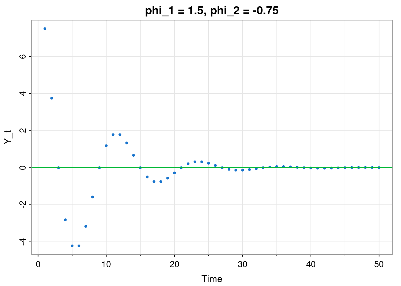

We could try solving this directly by looking for solutions of the form \(y_t = A\lambda^t\). Substituting in leads to the quadratic \[ \lambda^2 - \phi_1\lambda - \phi_2 = 0. \] This will have two solutions, \(\lambda_1, \lambda_2\), leading to a general solution of the form \[ y_t = A_1\lambda_1^t + A_2\lambda_2^t, \] (assuming that \(\lambda_1\not= \lambda_2\)), and the two initial values \(y_0, y_1\) can be used to deduce the values of \(A_1, A_2\). It is clear that this solution will be stable provided that \(|\lambda_i|<1\), \(i=1, 2\).

Which combinations of \(\phi_1\) and \(\phi_2\) will lead to stable systems? Since we have a condition on \(\lambda_i\) and the \(\lambda_i\) are just a function of \(\phi_1\) and \(\phi_2\), we can figure out the region of \(\phi_1\)–\(\phi_2\) space corresponding to stable solutions. Careful analysis of the relevant inequalities reveals that the stable region is the triangular region defined by \[ \phi_2 < 1-\phi_1,\quad \phi_2 < 1 + \phi_1,\quad \phi_2 > -1. \] Within this triangular region, \(\lambda_i\) will be complex if \(\phi_1^2 + 4\phi_2 < 0\), and this will correspond to the oscillatory stable region.

We can consider a shifted version (\(x_t = y_t + \mu\)), as before.

This is all fine, but an alternative is to re-write the system as a first order vector recurrence \[ \binom{y_t}{y_{t-1}} = \begin{pmatrix}\phi_1&\phi_2\\1&0\end{pmatrix}\binom{y_{t-1}}{y_{t-2}}. \] We know that this system will be stable provided that the eigenvalues of the update matrix lie inside the unit circle. We can check that the eigenvalues of this matrix are given by the solutions of the quadratic in \(\lambda\) considered above. This technique of taking a higher-order linear dynamical system and expressing it as a first order system with a higher-dimensional state space can be applied to all of the models that we have been considering: deterministic or stochastic, discrete or cts time.

2.4.1.2 Vector discrete time

The second-order vector discrete time linear recursion \[ \mathbf{y}_t = \mathsf{\Phi}_1\mathbf{y}_{t-1} + \mathsf{\Phi}_2\mathbf{y}_{t-2} \] can be re-written as the first order system \[ \binom{\mathbf{y}_t}{\mathbf{y}_{t-1}} = \begin{pmatrix}\mathsf{\Phi}_1&\mathsf{\Phi}_2\\\mathbb{I}&0\end{pmatrix} \binom{\mathbf{y}_{t-1}}{\mathbf{y}_{t-2}}. \]

2.4.1.3 Continuous time

The scalar second-order linear system in cts time can be written \[ \ddot y + \nu_1\dot y + \nu_2 y = 0, \] and initialised with \(y(0)\) and \(\dot y(0)\). Here, when compared to the first-order equivalent, there has been a switch of parameter from \(\lambda\) to \(\nu_1,\nu_2\) in order to avoid confusion with eigenvalues. As with the discrete time system, we could directly analyse this system by looking for solutions of the form \(y=Ae^{\lambda t}\). Substituting in leads to the quadratic \[ \lambda^2 + \nu_1\lambda + \nu_2 = 0. \] This can be solved for the two solutions \(\lambda_1, \lambda_2\) to get a general solution of the form \[ y(t) = A_1e^{\lambda_1 t} + A_2e^{\lambda_2 t} \] (assuming that \(\lambda_1 \not= \lambda_2\)), and the initial conditions can be used to solve for \(A_1, A_2\). It is clear that this system will be stable provided that the real parts of \(\lambda_1,\lambda_2\) are both negative.

Alternatively, by defining \(v\equiv \dot y\), this second-order system could be re-written as \[ \dot v + \nu_1 v + \nu_2 y = 0, \] and hence as the first order vector system, \[ \binom{\dot v}{\dot y} = \begin{pmatrix}-\nu_1&-\nu_2\\1&0\end{pmatrix} \binom{v}{y}. \] We know that this system will be stable provided that the generator matrix has eigenvalues with negative real parts. Solving for the eigenvalues leads to the same quadratic in \(\lambda\) we deduced above.

We can consider the stable region in terms of \(\nu_1\) and \(\nu_2\). Again, careful analysis of the relevant inequalities reveals that the stable region corresponds to the positive quadrant \(\nu_1,\nu_2>0\), and that the roots will be complex if \(4\nu_2 > \nu_1^2\).

2.4.1.4 Vector continuous time

The second-order vector linear system \[ \ddot{\mathbf{y}} + \mathsf{\Lambda}_1\dot{\mathbf{y}} + \mathsf{\Lambda}_2 \mathbf{y} = \mathbf{0}, \] can be re-written as the first-order system \[ \binom{\dot{\mathbf{v}}}{\dot{\mathbf{y}}} = \begin{pmatrix}-\mathsf{\Lambda}_1&-\mathsf{\Lambda}_2\\\mathbb{I}&0\end{pmatrix} \binom{\mathbf{v}}{\mathbf{y}}, \] where \(\mathbf{v}\equiv\dot{\mathbf{y}}\).

2.4.2 Stochastic

2.4.2.1 Discrete time: AR(2)

The second-order Markovian scalar linear Gaussian auto-regressive model, AR(2), takes the form \[ Y_t = \phi_1Y_{t-1} + \phi_2Y_{t-2} + \varepsilon_t,\quad \varepsilon_t\sim \mathcal{N}(0,\sigma^2). \]

tsplot(filter(rnorm(80), c(1.5, -0.75), "rec", init=c(20,20)),
  type="p", pch=19, col=4, cex=0.5, ylab="Y_t",
  main="phi_1 = 1.5, phi_2 = -0.75")
abline(h=0, col=3, lwd=2)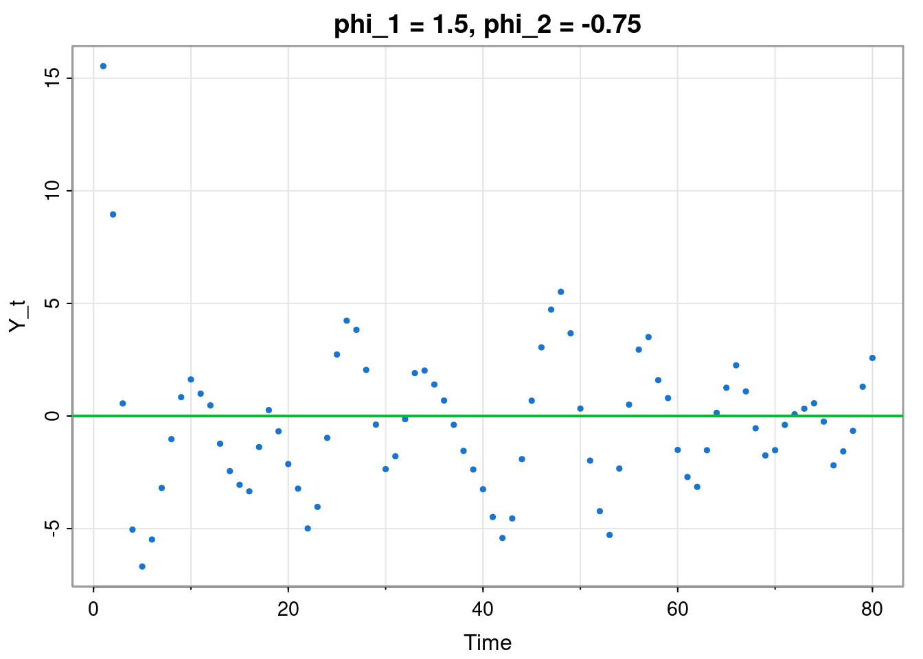

Taking expectations gives the second-order linear recurrence \[ \mathbb{E}[Y_t] = \phi_1\mathbb{E}[Y_{t-1}] + \phi_2\mathbb{E}[Y_{t-2}]. \] Looking for solutions of the form \(\mathbb{E}[Y_t]=A\lambda^t\) gives the quadratic \[ \lambda^2 - \phi_1\lambda-\phi_2=0, \] so the system will be stable if the solutions, \(\lambda_i\), are inside the unit circle (\(|\lambda_i|<1\)). We have already described this stable region in \(\phi_1\)–\(\phi_2\) space, while examining the deterministic second-order linear recurrence.

Alternatively, we could re-write this second-order system as the VAR(1): \[ \binom{Y_t}{Y_{t-1}} = \begin{pmatrix}\phi_1&\phi_2\\1&0\end{pmatrix}\binom{Y_{t-1}}{Y_{t-2}} + \binom{\varepsilon_t}{0}. \] We know that this system will be stable if the eigenvalues of the auto-regressive matrix are inside the unit circle. But solving for the eigenvalues leads to the same quadratic that we deduced above. Also note that here the error variance matrix is \(\begin{pmatrix}\sigma^2&0\\0&0\end{pmatrix}\).

2.4.2.2 Vector discrete time: VAR(2)

The VAR(2) model \[ \mathbf{Y}_t = \mathsf{\Phi}_1\mathbf{Y}_{t-1} + \mathsf{\Phi}_2\mathbf{Y}_{t-2} + \pmb{\varepsilon}_t,\quad \pmb{\varepsilon}_t\sim N(\mathbf{0},\mathsf{\Sigma}) \] can be re-written as the VAR(1) system \[ \binom{\mathbf{Y}_t}{\mathbf{Y}_{t-1}} = \begin{pmatrix}\mathsf{\Phi}_1&\mathsf{\Phi}_2\\\mathbb{I}&0\end{pmatrix}\binom{\mathbf{Y}_{t-1}}{\mathbf{Y}_{t-2}} + \binom{\pmb{\varepsilon}_t}{\mathbf{0}}. \] It will be stable when the eigenvalues of the auto-regressive matrix lie inside the unit circle.

2.4.2.3 Continuous time

We wrote the first-order continuous time linear system in the form \[ \mathrm{d}Y(t) = -\lambda Y(t)\,\mathrm{d}t + \sigma\,\mathrm{d}W(t), \] where \(W(t)\) is a Wiener process, but a physicist might just write it as a Langevin equation: \[ \dot Y(t) + \lambda Y(t) = \sigma \eta(t), \] where \(\eta(t)\) is a “white noise” process. This requires some care in interpreting, since \(Y(t)\) is not actually differentiable, and \(\eta(t)\) is not a regular function. However, this way of writing it makes the second-order generalisation more obvious: \[ \ddot Y(t) + \nu_1\dot Y(t) + \nu_2 Y(t) = \sigma\eta(t), \] where, again, we’ve switched from \(\lambda\) to \(\nu_i\) to avoid confusion with eigenvalues. If we throw caution to the wind, take expectations, and put \(m(t) = \mathbb{E}[Y(t)]\) we get \[ \ddot m + \nu_1\dot m + \nu_2 = 0. \] We know that seeking solutions of the form \(m(t)=Ae^{\lambda t}\) will lead to the quadratic \[ \lambda^2 + \nu_1 \lambda +\nu_2 = 0 \] and that the system will be stable provided that the solutions, \(\lambda_i\), both have negative real part.

If we now try to be a bit more careful, and define \(V(t)=\dot Y(t)\), we can re-write the Langevin equation as \[ \dot{V}(t) + \nu_1 V(t) + \nu_2 Y(t) = \sigma\eta(t), \] and then it is reasonably clear that we can write the system as a pair of coupled (S)DEs, \[\begin{align*} \mathrm{d}V(t) &= -(\nu_1 V(t) + \nu_2Y(t))\mathrm{d}t + \sigma\,\mathrm{d}W(t) \\ \mathrm{d}Y(t) &= V(t)\,\mathrm{d}t, \end{align*}\] and hence as a first-order vector OU process \[ \binom{\mathrm{d}V(t)}{\mathrm{d}Y(t)} = \begin{pmatrix}-\nu_1&-\nu_2\\1&0\end{pmatrix}\binom{V(t)}{Y(t)}\mathrm{d}t + \begin{pmatrix}\sigma&0\\0&0\end{pmatrix}\binom{\mathrm{d}W_{1,t}}{\mathrm{d}W_{2,t}}. \] We know that this VOU process will be stable if the eigenvalues of the generator matrix have negative real parts, but of course, solving for the eigenvalues leads to the quadratic we deduced above.

2.4.2.4 Vector continuous time

Using “physics notation”, we could informally write the second-order system as \[ \ddot{\mathbf{Y}}(t) + \mathsf{\Lambda}_1\dot{\mathbf{Y}}(t) + \mathsf{\Lambda}_2\mathbf{Y}(t) = \mathsf{\Omega}\,\pmb{\eta}(t), \] understanding that what this really represents is the VOU process \[ \binom{\mathrm{d}\mathbf{V}(t)}{\mathrm{d}\mathbf{Y}(t)} = \begin{pmatrix}-\mathsf{\Lambda}_1&-\mathsf{\Lambda}_2\\\mathbb{I}&0\end{pmatrix}\binom{\mathbf{V}(t)}{\mathbf{Y}(t)}\mathrm{d}t + \begin{pmatrix}\mathsf{\Omega}&0\\0&0\end{pmatrix}\binom{\mathrm{d}\mathbf{W}_{1,t}}{\mathrm{d}\mathbf{W}_{2,t}}, \] where \(\mathbf{V}(t)=\dot{\mathbf{Y}}(t)\). Stability can be determined by checking if the eigenvalues of the generator matrix all have negative real part.