A spatio-temporal data set is just a collection of observations labelled in both time and space. So \(x(\mathbf{s}; t)\) is an observation at location \(\mathbf{s}\in\mathcal{D}\) at time \(t\in\mathbb{R}\). The spatial domain, \(\mathcal{D}\), is usually a subset of \(\mathbb{R}^2\) or \(\mathbb{R}^3\). You have seen in the first term that there are a huge range of different kinds of spatial data, and that different models and methods are appropriate for different situations. The range of different kinds of spatio-temporal models and data is even greater. We do not have time to explore these in detail now. Here we need to concentrate on the most commonly encountered form of spatio-temporal data. That is, data consisting of scalar-valued time series on a regular time grid of length \(n\) being observed at a fixed collection of irregularly distributed sites, of which there are \(m\). We could write \(\mathbf{x}(\mathbf{s})\) for the time series at site \(\mathbf{s}\in\mathcal{D}\), \(\mathcal{D}=\{\mathbf{s}_1,\ldots,\mathbf{s}_m\}\). We assume for now that we have temporally aligned time series across the sites, leading to a “full grid” of spatio-temporal data. That is, we have \(nm\) scalar observations, \[
\{x(\mathbf{s}_i; t)\ |\ i=1,\ldots,m,\ t=1,\ldots,n\}.
\] For data of this form on a regular time grid, we often use the notation \(x_t(\mathbf{s})\) for \(x(\mathbf{s};t)\), and sometimes write \(\mathbf{x}_t=(x_t(\mathbf{s}_1),\ldots,x_t(\mathbf{s}_m))^\top\) for the realisation of the spatial process at time \(t\). We could also write \(\mathsf{X}\) for the \(n\times m\) matrix with \((i,j)\)th element \(x_i(\mathbf{s}_j)\). When the data matrix is arranged this way it is said to be in “space-wide” format. \(\mathsf{X}^\top\) is said to be in “time-wide” format. In practice, it is rare to actually have all \(nm\) observations of this form, but we can often represent our data in this form provided that we are allowed to have missing data. In general, strategies are needed to deal with missing spatio-temporal observations.
We immediately see that there are two different ways of “slicing” data of this form, and these correspond to different modelling perspectives. If we adopt the spatial perspective, we regard the data as spatial, but with a multivariate observation at each site that happens to be a time series. We can then adopt spatial approaches to model the cross-correlation between the time series at different sites. This spatial perspective underpins many classical approaches to spatio-temporal modelling, but has limitations that we don’t have time to fully explore in this module. The alternative dynamic or temporal perspective, views the data as a time series, where the multivariate observation at each time happens to be the realisation of a spatial process. This latter approach is in many ways more satisfactory, and underpins many modern approaches to spatio-temporal modelling.
9.2 Exploring spatio-temporal data
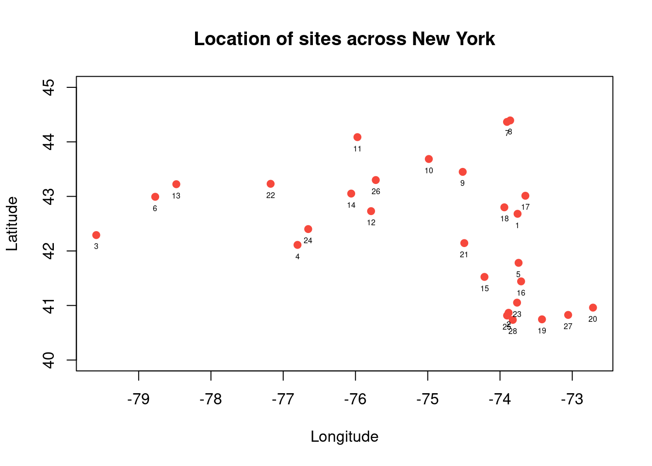
Before proceeding further, it will be useful to familiarise ourselves with some spatio-temporal data. Our main running example for this chapter will be the dataset spTimer::NYdata, some air quality data, measured over time, at a collection of locations across New York. You can find out more about the spTimer package with help(package="spTimer"). Let’s start by trying to understand the basic structure of the data.
We can see straight away that the data is currently in “long format”, where observations (of several different variables) are recorded with both a position in space and time. You can find out more about the data with ?NYdata. Let us proceed by finding out more about the sites.
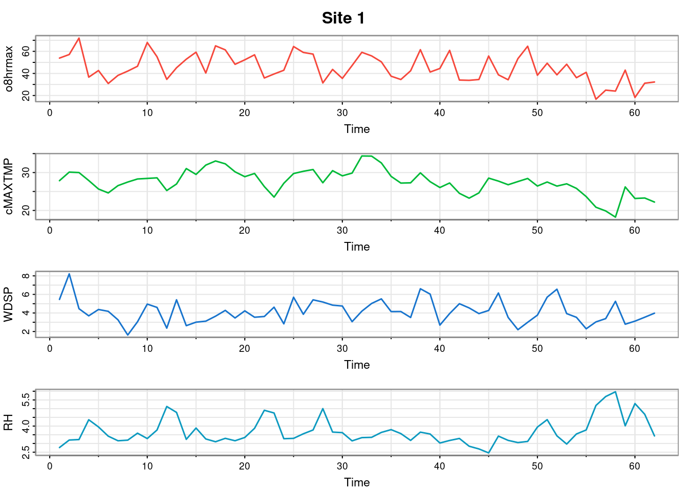
So the observations in space and time are actually multivariate, with several different variables begin measured simultaneously. To keep things simpler, we will focus on just one variable, ozone.
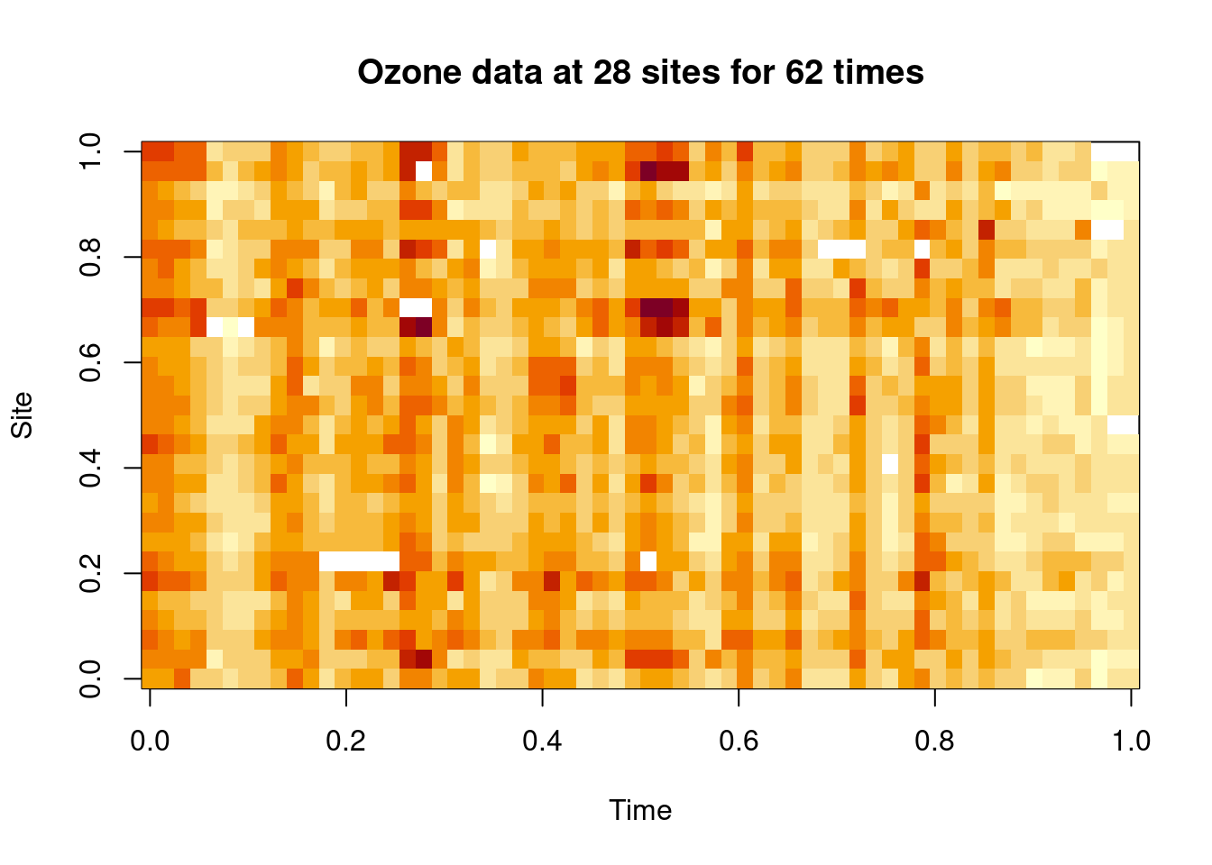
ozone=NYdata[,c("o8hrmax", "s.index")]ozone=unstack(ozone)dim(ozone)# "space-wide" format
[1] 62 28
## "full grid" representation - "STF" in "spacetime" terminologyimage(as.matrix(ozone), main="Ozone data at 28 sites for 62 times", xlab="Time", ylab="Site")
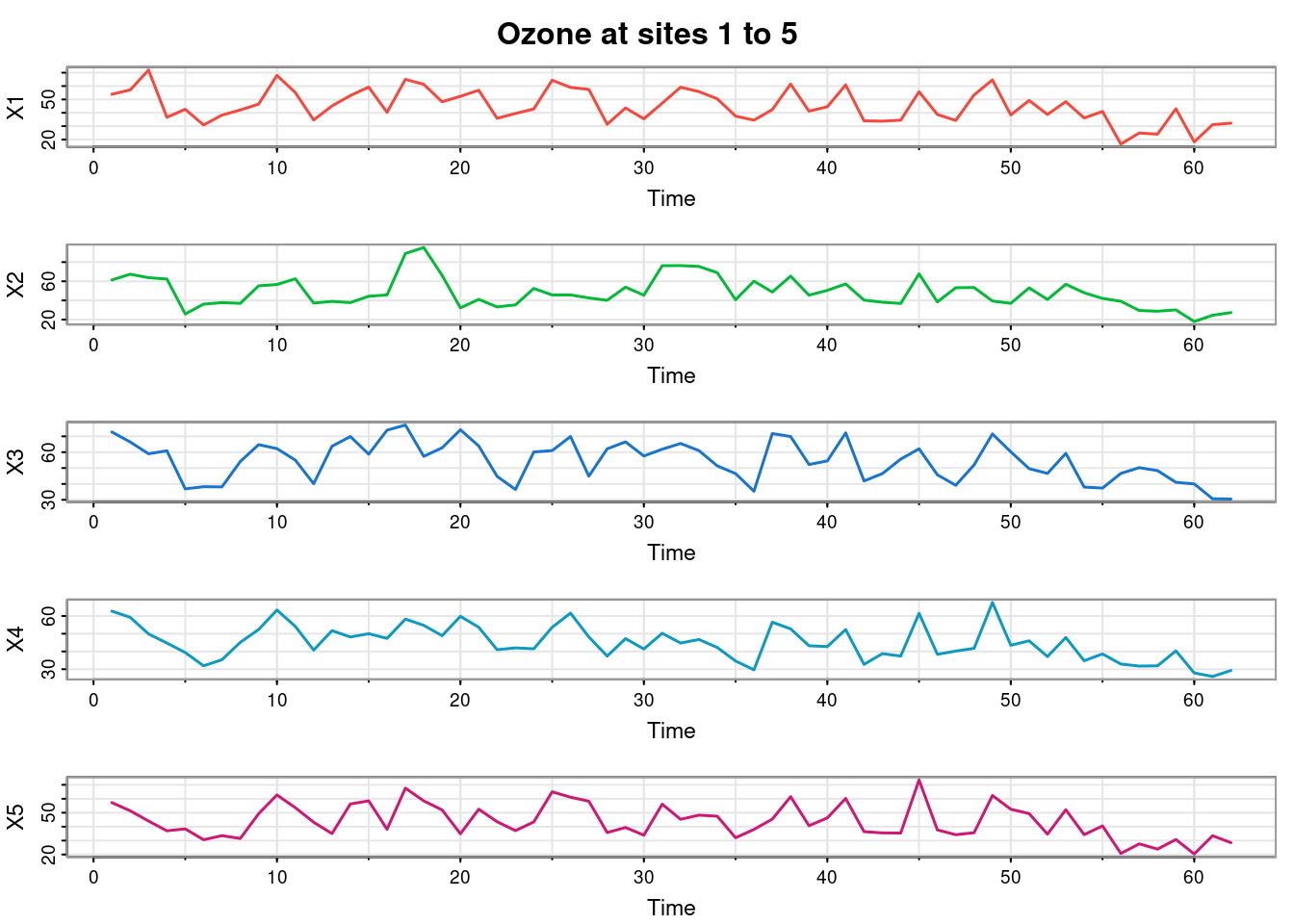
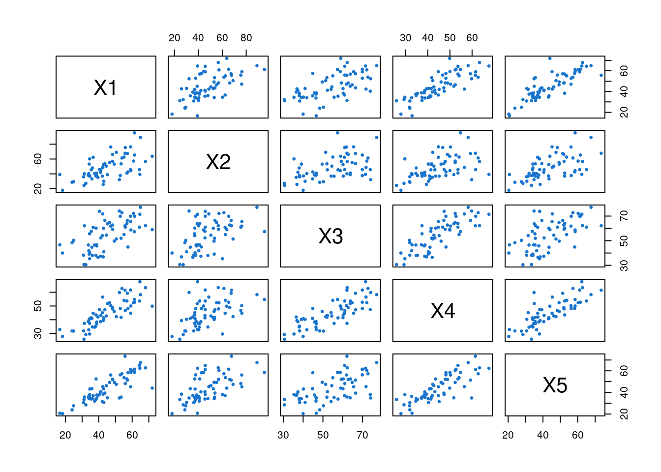
We can visualise the data matrix as an image, which shows a few missing observations (in white), but not too many. This is a fairly complete full-grid spatio-temporal dataset. We can do time series plots for a very small number of sites at once.
tsplot(ozone[,1:5], col=2:6, lwd=1.5,
  main="Ozone at sites 1 to 5")
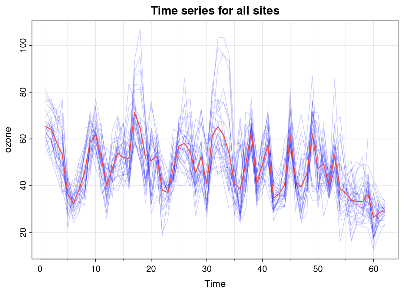
But to look at the time series for all sites simultaneously, we need to overlay, and use transparency to stop the plot from looking too messy.
tsplot(ozone, spaghetti=TRUE, col=rgb(0, 0, 1, 0.2), ylab="ozone", main="Time series for all sites")lines(rowMeans(ozone, na.rm=TRUE), col=2, lwd=1.5)
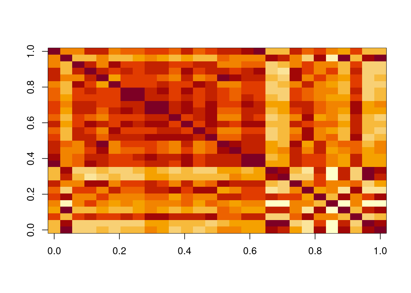
Similarly, we can look in detail at cross-correlations for a small number of time series, but need to revert to an image to see the full correlation structure.
It is clear from this that there is a lot of interesting correlation structure present, but we are not currently doing anything with the highly relevant context of spatial proximity.
9.3 Spatio-temporal modelling
9.3.1 Spatial models
We begin by taking a more spatial view of spatio-temporal data. So, now we have a time series at a collection of sites. We could completely ignore the temporal dependence and regard the observations at each time as being iid realisations of a spatial process, or we could regard time as an additional dimension. We begin with the former view.
9.3.1.1 Purely spatial models
We begin by ignoring temporal dependence completely, so that observations at each time are independent realisations of some multivariate distribution representing the spatial process.
9.3.1.1.1 Unconstrained multivariate data
If we know nothing about the spatial context, we can just regard the observations at each time point as being multivariate normal, \[
\mathbf{X}_t \sim \mathcal{N}(\mathbf{0}, \mathsf{\Sigma}),
\] for unconstrained \(\mathsf{\Sigma}\), after stripping out any mean. Then the sample covariance matrix of the data estimates \(\mathsf{\Sigma}\).
Unconstrained estimation of the covariance matrix is potential problematic, since it has a very large number of degrees of freedom, and we are not exploiting our known spatial context. So we probably prefer to regard the observations as being iid from a Gaussian process (GP) with a parameterised covariance function. Here, for simplicity, we will use an isotropiccovariance function, depending only on the geographical distance between the sites. Here, for illustrative purposes, we will use the squared exponential covariance function \[
C(d) = \sigma^2\exp\{-d^2/a^2\}, \quad \sigma,a>0,
\] with \(\sigma^2\) representing the stationary variance of the GP, and \(a\) the length scale. We can encode this in R with
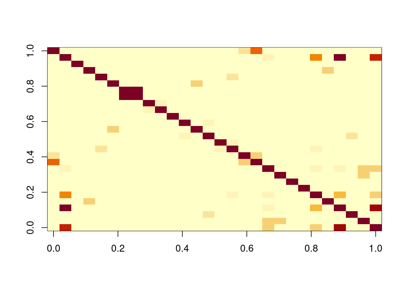
suggesting a length scale of around 30km for ozone. We also see that the optimal covariance matrix looks quite different to the sample covariance matrix, and that there is very little correlation between sites that are not very close together (such as sites 7 and 8). This is good and bad. It is good that it properly spatially smooths, but the assumption of a common variance across sites is probably not realistic.
9.3.1.2 Space-time Gaussian process models
Ignoring the temporal dependence structure in the data is obviously unsatisfactory for various reasons. If we persist with our spatial-first perspective, we consider the presence of a time series at each spatial location. This time series could potentially also be modelled as a GP. If we think that a GP is appropriate for both spatial and temporal variation, and that the same GP model is appropriate for every time series irrespective of spatial location, then we are led to modelling the data in space and time as arising jointly from a single GP with a separable space-time covariance function of the form \[
C(\mathbf{s},t) = C_s(\mathbf{s})C_t(t),
\] for given spatial covariance function \(C_s(\cdot)\) and temporal covariance function \(C_t(\cdot)\). Adopting a separable covariance function is convenient for multiple reasons. First, if \(C_s\) is a valid spatial covariance function and \(C_t\) is a valid temporal covariance function, then their product is guaranteed to be a valid space-time covariance function. Thus, the imposition of separability greatly simplifies the specification of a valid spatio-temporal covariance function. Second, the assumption greatly simplifies computation, since then the joint covariance matrix over all observations can be represented as a Kronecker product of the spatial and temporal covariance matrices, allowing the avoidance of the construction or inversion of very large matrices.
Much of classical spatio-temporal modelling was built on separable GP models. However, it turns out that the assumption of separability is very strong, and quite unrealistic for most spatio-temporal data sets. So, given our limited time, we will abandon this approach, and adopt a more dynamical perspective.
9.3.2 Dynamic models for spatio-temporal data
This term we have studied models for time series, and in particular, ARMA models, and DLMs. Both of these families of models lead to linear Gaussian systems. They therefore determine Gaussian process models, and implicitly determine a (not necessarily stationary) covariance structure. However, we don’t specify these models via their covariance structure. We specify their dynamics, and the dynamics implicitly determines the covariance structure. There are many advantages to this more dynamical perspective.
9.3.2.1 Random walk model
We will begin with a model that is typically over-simplistic, but we will gradually refine and improve it. Rather than assuming that our observations are iid, we will assume that they form a random walk \[
\mathbf{X}_t = \mathbf{X}_{t-1} + \pmb{\varepsilon}_t,\quad \pmb{\varepsilon}_t\sim \mathcal{N}(\mathbf{0},\mathsf{\Sigma}).
\] This non-stationary model will sometimes be appropriate when there is a high degree of persistence in changes to the levels observed. This model is very simple to fit, since the one-step differences are iid, so we can put \[
\pmb{\varepsilon}_t = \mathbf{X}_t - \mathbf{X}_{t-1},
\] and estimate the parameters of iid \(\pmb{\varepsilon}_t\) as for the iid model. Again, we could have an unconstrained \(\mathsf{\Sigma}\), which we can estimate using the sample covariance matrix of the one-step differences, or a constrained matrix, with an explicitly spatial covariance structure, which we can estimate via maximum likelihood, as we have already seen.
9.3.2.2 VAR(1) models
We can greatly improve on the simple random walk model by allowing VAR(1) dynamics, assuming temporal evolution of the form \[
\mathbf{X}_t = \mathsf{G}\mathbf{X}_{t-1} + \pmb{\varepsilon}_t,\quad \pmb{\varepsilon}_t\sim \mathcal{N}(\mathbf{0},\mathsf{\Sigma}),
\] perhaps following some mean-centring. This model is specified by \(m\times m\) matrices \(\mathsf{G}\) and \(\mathsf{\Sigma}\). This model is very flexible, allowing a range of different stationary and non-stationary dynamics. But the utility of the model depends crucially on having an appropriate structure for the propagator matrix, \(\mathsf{G}\). Clearly, choosing \(\mathsf{G}=\mathbb{I}\) gives the random walk model we have already considered, so this model class includes the random walk model as a special case.
9.3.2.2.1 Unconstrained models
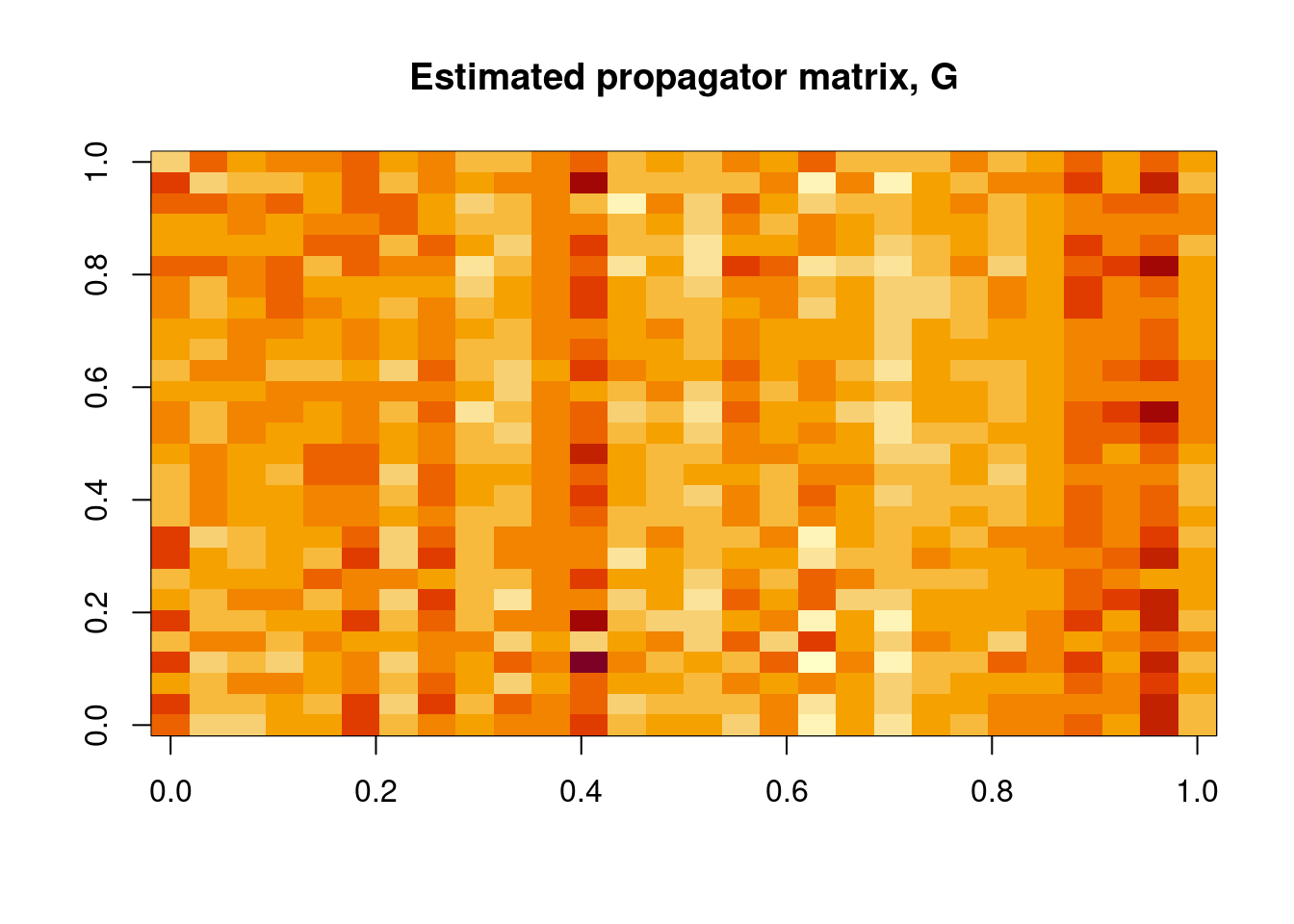
Obviously, one possibility is to consider a completely unconstrained \(\mathsf{G}\), with elements to be estimated by least squares (or maximum likelihood). We can use the same least squares approach that we adopted in Chapter 4 by writing our model in the form \[
\mathsf{X}_{2:n} = \mathsf{X}_{1:(n-1)}\mathsf{G}^\top+ \mathsf{E},
\] to get the least squares solution \[
\hat{\mathsf{G}}^\top= ( \mathsf{X}_{1:(n-1)}^\top\mathsf{X}_{1:(n-1)})^{-1} \mathsf{X}_{1:(n-1)}^\top\mathsf{X}_{2:n}.
\]
Once we know \(\mathsf{G}\) we can estimate \(\mathsf{\Sigma}\) conditional on \(\mathsf{G}\) as discussed for the random walk model. Note that there is no reason to expect (or want) \(\mathsf{G}\) to be symmetric, and there is also no reason why all of the elements should be non-negative. Clearly this approach could be used for any multivariate time series, so we are not properly exploiting the spatial context. Also, for a large number of sites, it can be problematic to estimate all \(m^2\) elements of \(\mathsf{G}\) given at most \(nm\) data points.
9.3.2.2.2 Diagonal propagation
As a compromise between a simple random walk model and a completely unconstrained propagation matrix, a diagonal \(\mathsf{G}\) can be assumed. This also ignores the spatial context, but nevertheless fixes a number of issues with the simple random walk model. Since \(\mathsf{G}\) is diagonal, from a least squares perspective the problem reduces to \(m\) independent AR(1) models that can be fit separately.
Alternatively, the problem can be set up as a least squares problem for the \(m\)-vector \(\mathbf{g}\), where \(\mathsf{G}=\operatorname{diag}\{\mathbf{g}\}\). This is tractable, with solution \[
\hat{\mathbf{g}} = \left(\sum_{t=2}^n \mathbf{x}_{t-1}\circ \mathbf{x}_t\right)
\circ \left(\sum_{t=2}^n \mathbf{x}_{t-1}\circ \mathbf{x}_{t-1}\right)^{-1}.
\]
Here, the solution using arima is preferred, since it has more intelligent handling of missing data.
9.3.2.2.3 Spatial mixing kernels
Ideally, we would like to use a propagator matrix, \(\mathsf{G}\), which takes into account the spatial context. This is relatively simple when the sites lie on a regular lattice (see the later discussion of STAR models), but more challenging for irregularly distributed spatial locations. Note that the \(i\)th row of \(\mathsf{G}\) corresponds to the weights applied to the sites at the previous time point when making a prediction for site \(i\) at the current time point. The diagonal model puts all weight on just site \(i\). It might be better to distribute the weights across the \(k\) nearest neighbours of site \(i\) for some reasonably small \(k>1\). Choosing a small \(k\) will ensure that most of the elements of \(\mathsf{G}\) are zero, and hence \(\mathsf{G}\) will be a sparse matrix, which has significant computational advantages. However, for fairly small \(m\) we could assume a dense \(\mathsf{G}\), with weights varying as a function of distance. It is common to assume some sort of kernel distance function, and there are many possible choices with various advantages and disadvantages. For example, we could use the squared exponential kernel (irrespective of any covariance kernel assumed for \(\mathsf{\Sigma}\)), \[
g_{ij} = \sigma_i\exp\{-\Vert \mathbf{s}_j-\mathbf{s}_i\Vert^2/a_i^2\}.
\] It is quite common (but not required) to assume that the length scale is common across all sites, \(a_i = a\). However, there are often very good reasons to allow \(\sigma_i\) to vary across sites, and in this case \(\mathsf{G}\) will not be symmetric (which is fine).
Given this parameterisation of \(\mathsf{G}\), and most likely also a low-dimensional parameterisation of \(\mathsf{\Sigma}\), it is straightforward to evaluate the Gaussian likelihood, and hence optimise the log-likelihood to find the optimal parameters, similar to what we have seen many times previously.
9.3.3 Dynamic latent process models
The spatio-temporal models that we have examined so far have all been special cases of the VAR(1) model. However, when we studied DLMs in Chapter 7, we saw that it can often make sense to assume a latent process of auto-regressive form, but to then model our observations as some noisy linear transformation of this hidden latent process. This remains the case in the spatio-temporal context. So it is natural to consider models of DLM form for spatio-temporal processes, \[\begin{align*}
\mathbf{Y}_t &= \mathsf{F}\mathbf{X}_t + \pmb{\nu}_t, \quad \pmb{\nu}_t\sim \mathcal{N}(\mathbf{0},\mathsf{V}) \\
\mathbf{X}_t &= \mathsf{G}\mathbf{X}_{t-1} + \pmb{\omega}_t.\quad \pmb{\omega}_t \sim \mathcal{N}(\mathbf{0},\mathsf{W}),
\end{align*}\] where \(\mathbf{Y}_t\) is our spatial observation at time \(t\), and \(\mathbf{X}_t\) is some kind of latent process representation of the underlying system state at time \(t\). The precise nature of the latent process can vary according to the modelling approach adopted. We briefly consider three possibilities.
9.3.3.1 Spatial mixing kernels
If we choose \(\mathsf{F}=\mathbb{I}\), then our observations are just random corruptions of the hidden latent state. So the latent state has a very similar interpretation as the models we have been considering so far. In particular, there is a one-to-one correspondence between sites and elements of the latent process state vector, and \(\mathsf{G}\) has an interpretation as a spatial mixing kernel for the hidden latent process. It can be parameterised in the manner previously discussed. A spatial covariance kernel is often used to parameterise \(\mathsf{W}\), and \(\mathsf{V}\) is often assumed to be diagonal. We have seen how to evaluate the log-likelihood of a DLM, so we can optimise the parameters of the kernel functions using maximum likelihood in the usual way.
9.3.3.2 Example: NY ozone data
Let’s see how we could implement a model like this using the dlm R package. To keep things simple we will just assume a propagator matrix of the form \(\mathsf{G}=\alpha\mathbb{I}\). We will also start off with an evolution covariance matrix of the form \(\mathsf{W} = \sigma_w^2\mathbb{I}\), but we will relax this assumption soon. We can fit this as follows.
library(dlm)buildMod=function(param){alpha=exp(param[1]); sigW=exp(param[2])sigV=exp(param[3])dlm(FF=diag(numSites), GG=alpha*diag(numSites), V =(sigV^2)*diag(numSites), W =(sigW^2)*diag(numSites), m0 =rep(0, numSites), C0 =(1e07)*diag(numSites))}opt=dlmMLE(as.matrix(cOzone), parm=log(c(0.8, 1, 3.0)), build=buildMod)opt
This works, and give smoothed states that are visibly smoother than the raw data. Importantly, it also sensibly smooths over the missing data. But this model isn’t really explicitly spatial. Apart from assuming common parameters across sites, the DLMs at each site are independent. For spatial smoothing we really want \(\mathsf{W}\) to be a spatial covariance matrix. We can fit a model using a spatial variance matrix of the form previously discussed (using our function cm) as follows.
This also works, after a fashion, but note that the optimal length scale is just the upper bound I imposed on the optimiser. If an upper bound is not imposed, the length scale just keeps increasing until the model crashes. Inferring length scales is notoriously difficult in spatial statistics, and is even more challenging in the spatio-temporal setting. So, given that in the context of purely spatial modelling we previously inferred a length scale of around 30km, we could just use that length scale in the context of the dynamic model and not try to optimise it.
buildMod=function(param){alpha=exp(param[1]); sigW=exp(param[2])sigV=exp(param[3])dlm(FF=diag(numSites), GG=alpha*diag(numSites), V =(sigV^2)*diag(numSites), W =cm(c(sigW, 30)), m0 =rep(0, numSites), C0 =(1e07)*diag(numSites))}opt=dlmMLE(as.matrix(cOzone), parm=c(log(0.8), log(1), log(3.0)), build=buildMod)opt
This is better. This is now giving us a dynamic model that can smooth in both time and space jointly.
9.3.3.3 STAR models
It has previously been mentioned that choosing the form of the propagator matrix, \(\mathsf{G}\), would be more straightforward if the spatial locations all lay on a regular lattice (typically, in 2d or 3d). Even if our actual observations \(\mathbf{Y}_t\) do not, we could nevertheless model the latent state, \(\mathbf{X}_t\), as a lattice process. eg., in the 2d case, we could then let \(X_{t,i,j}\) be the value of the latent state at time \(t\) at position \((i,j)\) on the lattice. A nearest-neighbour model for the time evolution of the latent state might then take the form \[
X_{t,i,j} = \alpha X_{t-1,i,j} + \beta(X_{t-1,i-1,j} + X_{t-1,i+1,j} + X_{t-1,i,j-1} + X_{t-1,i,j+1} ) + \omega_{t,i,j},
\] for some fixed \(\alpha,\beta>0\). For stability, we might require \(\alpha+4\beta<1\). This then determines the sparse structure of \(\mathsf{G}\). There are many possible variations on this approach. \(\mathsf{W}\) could be diagonal or parameterised via a spatial covariance kernel. \(\mathsf{V}\) is often assumed to be diagonal. Models of this form are known as space-time auto-regressive models of order one, or STAR(1), and there are generalisations to higher order, STAR(p).
The matrix \(\mathsf{F}\) maps the actual observation sites onto the lattice. It will have \(m\) rows, and the number of columns will match the total number of sites on the lattice. The \(i\)th row of \(\mathsf{F}\) will have a 1 in the position corresponding to the lattice site closest to \(\mathbf{s}_i\), and zeros elsewhere.
DLM smoothing with this model allows interpolation of the observed data onto a regular space-time lattice. However, if the size of the lattice is large, this is computationally very demanding (notwithstanding the sparsity of \(\mathsf{G}\)). There are other possible approaches to spatio-temporal smoothing and interpolation which may be less computationally demanding.
9.3.3.4 Basis models (spectral approaches)
STAR models provide one approach to interpolate the hidden spatio-temporal process to spatial locations other than those that have been directly observed. STAR models are typically used in order to interpolate onto a regular lattice. However, there is no reason why we can’t construct a DLM that allows interpolation onto a continuous space. We just need some basis functions, for example, 2d or 3d Fourier basis functions. So, let \[
\phi_j: \mathbb{R}^2 \rightarrow \mathbb{R}, \quad j=1,2,\ldots
\] be basis functions defined on the whole of \(\mathbb{R}^2\) (or \(\mathbb{R}^3\) for 3d data). The idea is that we can represent an arbitrary function \(\theta:\mathbb{R}^2\rightarrow\mathbb{R}\) with an appropriate linear combination of basis functions \[
\theta(\mathbf{s}) = \sum_{j=1}^\infty \phi_j(\mathbf{s})x_j,
\] for some collection of coefficients \(x_1,x_2,\ldots\). We will seek a reduced dimension representation of a function by using just \(p\) basis functions. We will typically choose \(p<m\), the number of sites with observations. Then, every \(p\)-vector \(\mathbf{x}=(x_1,\ldots,x_p)^\top\) determines a function \[
\theta(\mathbf{s}) = \sum_{j=1}^p \phi_j(\mathbf{s})x_j,
\] If we allow \(\mathbf{x}\) to evolve in time, then the function \(\theta(\cdot)\) that it represents will also evolve in time. So, we can let the coefficient vector evolve according to \[
\mathbf{X}_t = \mathsf{G}\mathbf{X}_{t-1} + \pmb{\omega}_t.\quad \pmb{\omega}_t \sim \mathcal{N}(0,\mathsf{W}),
\] for some very simple propagator matrix such as \(\mathsf{G}=\mathbb{I}\) or \(\mathsf{G}=\alpha\mathbb{I}\) for \(\alpha\in(0,1)\). Since we know from Chapter 5 that Fourier transforms decorrelate GPs, we can reasonably assume diagonal \(\mathsf{W}\).
We probably want an observation model of the form \[\begin{align*}
Y_{t,i} &= \theta_t(\mathbf{s}_i) + \nu_{t,i} \\
&= \sum_{j=1}^p \phi_j(\mathbf{s}_i)X_{t,j} + \nu_{t,i},
\end{align*}\] and so \(\mathsf{F}\) is the \(m\times p\) matrix with \((i,j)\)th element \(\phi_j(\mathbf{s}_i)\). Again, \(\mathsf{V}\) is often taken to be diagonal, but doesn’t have to be. This is now just a DLM with a small number of parameters that can be fit in the usual ways. If we compute the smoothed coefficients of the latent coefficient vectors, these can be used in conjunction with the basis functions to interpolate the hidden spatial process over continuous space.
There are many possible choices of basis functions that can be used. 2d or 3d Fourier basis functions are the most obvious choice, but cosine basis functions, or wavelet basis functions, or some kind of empirical eigenfunctions can all be used.
9.3.4 R software
Fitting dynamic spatio-temporal models to data gets quite complicated and computationally intensive quite quickly. Relevant R software packages are summarised in the spatio-temporal task view. The IDE package will fit an integro-difference equation model, which we have not explicitly discussed, but is closely related to the STAR and spectral approaches. This package, in addition to a number of other approaches to the analysis of spatio-temporal data using R, is discussed in Wikle, Zammit-Mangion, and Cressie (2019). Otherwise, packages such as spBayes and spTimer will fit spatio-temporal models from a Bayesian perspective, using MCMC. Unfortunately we do not have time to explore these packages properly in this course.
9.4 Example: German air quality data
For further spatio-temporal investigation, it will be useful to have a different dataset to explore. We will now look briefly at a larger dataset than the one we have considered so far, but detailed analysis is left as an exercise.
The data is air quality data (specifically, PM10 concentration), for 70 different sites in Germany, over a 10 year period. We can load and inspect the data as follows.
It is actually in “time-wide” format, which we don’t necessarily want, and can be logged to be more Gaussian.
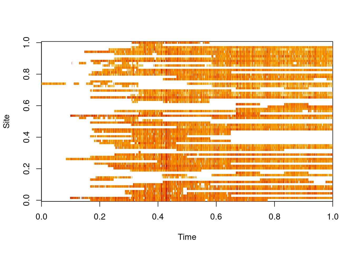
lair=t(log(air))# space-wide format (and logged)image(lair, xlab="Time", ylab="Site")# lots of missing data
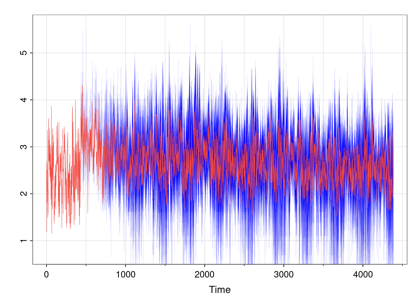
We see that there is a lot of missing data in this dataset, so a proper analysis will need to carefully handle missing data issues. We can attempt to overlay the time series at the different sites.
This is less satisfactory than for the New York data, but does give a reasonable overview of the dataset. The spacetime package has a special data structure for “full grid” spatio-temporal data like this, and we can create such a STF object as follows.
We are now in a position to think about how to apply our newly acquired spatio-temporal modelling skills to this dataset. Doing so is left as an exercise.
9.5 Wrap-up
This has been the briefest of introductions to spatio-temporal modelling. However, many of the most important concepts and issues have been touched upon, so this material will hopefully form a useful starting point for further study.
More generally, in this half of the module we have concentrated mainly on a dynamical approach to the modelling and analysis of temporal data, using model families such as ARMA, HMM and DLM. This dynamical view has many advantages over some more classical approaches to describing temporal data. Further, we have seen how this dynamical view often has computational advantages, typically leading to algorithms that have complexity that is linear in the number of time points. We have skimmed over many technical issues and details, and there is obviously a lot more to know. But again, I hope to have provided an intuitive introduction to many of the most important problems and concepts, and that you now have a better appreciation for random processes and data that evolve in (space and) time.
Wikle, C. K., A. Zammit-Mangion, and N. Cressie. 2019. Spatio-Temporal Statistics with R. CRC Press.