8 State space modelling
8.1 Introduction
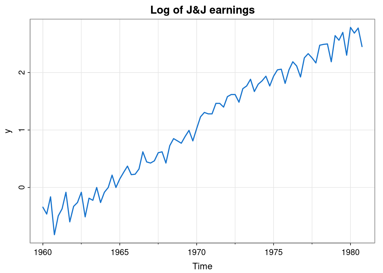
In Chapter 7 we introduced the DLM and showed how a model of DLM form could be used for filtering, smoothing, forecasting, etc. However, we haven’t yet discussed how to go about “building” an appropriate DLM model (in particular, specifying \(\mathsf{G}_t, \mathsf{F}_t, \mathsf{W}_t, \mathsf{V}_t\)) for a given time series. That is the topic of this chapter. We will use the dlm R package to illustrate the concepts. We will start by looking at some simple models for long-term trends, then consider seasonal effects, then the problem of combining trends and seasonal effects, before going on to think about the incorporation of ARMA components. We will focus mainly on (time invariant models for) univariate time series, but will briefly examine multivariate time series at the end of the chapter. Our main running example will be (the log of) J&J earnings, considered briefly in Chapter 1.
8.2 Polynomial trend
8.2.1 Locally constant model
In the previous chapter we saw that the choice \(\mathsf{G}=1\), \(\mathsf{F}=1\) corresponds to noisy observation of a Gaussian random walk. This random walk model for the underlying (hidden) state is known as the locally constant model in the context of DLMs, and sometimes (for reasons to become clear), as the first order polynomial trend model. Such a model is clearly inappropriate for the J&J example, since the trend appears to be (at least, locally) linear.
8.2.2 Locally linear model
We can model a time series with a locally linear trend by choosing \(\mathsf{F}=(1, 0)\), \[ \mathsf{G} = \begin{pmatrix}1&1\\0&1\end{pmatrix},\quad \mathsf{W}=\begin{pmatrix}w_1&0\\0&w_2\end{pmatrix}. \] This is known as the locally linear model, or sometimes as the second order polynomial trend model. To see why this corresponds to a linear trend, it is perhaps helpful to write the hidden state vector as \(\mathbf{X}_t=(\mu_t, \tau_t)^\top\). So then \(y_t\) is clearly just a noisy observation of \(\mu_t\) (the current level), and \(\mu_t=\mu_{t-1}+\tau_{t-1}+\omega_{1,t}\), so the current level increases by a systematic amount \(\tau_{t-1}\) (the trend), and is also corrupted by noise. On the other hand, \(\tau_t=\tau_{t-1}+\omega_{2,t}\) is just a random walk (typically with very small variance, so that the trend changes very slowly).
We can create such a model using the dlm::dlmModPoly function, by providing the order required (2 for locally linear), and the diagonal of \(\mathsf{V}\) and \(\mathsf{W}\) (off-diagonal elements are assumed to be zero).
mod = dlmModPoly(2, dV=0.1^2, dW=c(0.01^2, 0.01^2))
mod
$FF
[,1] [,2]
[1,] 1 0
$V
[,1]
[1,] 0.01
$GG
[,1] [,2]
[1,] 1 1
[2,] 0 1
$W
[,1] [,2]
[1,] 1e-04 0e+00
[2,] 0e+00 1e-04
$m0
[1] 0 0
$C0
[,1] [,2]
[1,] 1e+07 0e+00
[2,] 0e+00 1e+07ss = dlmSmooth(y, mod)
tsplot(y, col=4, lwd=2, main="Log of J&J earnings")
lines(ss$s[,1], col=2, lwd=2)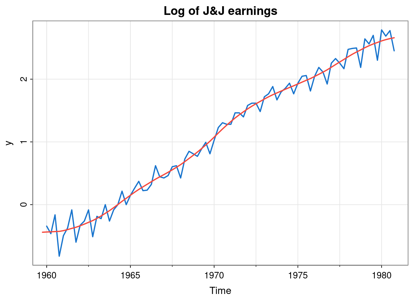
This captures the trend quite well, but not the strong seasonal effect. We will return to this issue shortly.
8.2.3 Higher-order polynomial models
This strategy extends straightforwardly to higher order polynomials. For example, a locally quadratic (order 3) model can be constructed using \(\mathsf{F}=(1,0,0)\) and \[ \mathsf{G} = \begin{pmatrix}1&1&0\\0&1&1\\0&0&1\end{pmatrix}. \] A diagonal \(\mathsf{W}\) is typically adopted, sometimes with some of the diagonal elements set to zero. Models beyond order 3 are rarely used in practice.
8.3 Seasonal models
Many time series exhibit periodic behaviour with known period. There are two commonly used approaches used to modelling such seasonal behaviour using DLMs. Both involve using a cyclic matrix, \(\mathsf{G}\), with period \(s\) (eg. \(s=12\) for monthly data), so that \(\mathsf{G}^s=\mathbb{I}\). We will look briefly at both.
8.3.1 Seasonal effects
Arguably the most straightforward way to model seasonality is to explicitly model \(s\) separate seasonal effects, and rotate and evolve them, as required. So, for a purely seasonal model, call the \(s\) seasonal effects \(\alpha_1,\alpha_2,\ldots,\alpha_s\), and make these the components of the state vector, \(\mathbf{X}_t\). Then choosing the \(1\times s\) matrix \(\mathsf{F}=(1,0,\ldots,0)\) and \(\mathsf{G}\) the \(s\times s\) cyclic permutation matrix \[ \mathsf{G} = \begin{pmatrix}\mathbf{0}^\top&1\\\mathbb{I}&\mathbf{0}\end{pmatrix} \] gives the basic evolution structure. For example, in the case \(s=4\) (quarterly data), we have \[ \mathsf{G} = \begin{pmatrix} 0&0&0&1\\ 1&0&0&0\\ 0&1&0&0\\ 0&0&1&0\end{pmatrix}, \] and so \[ \mathsf{G}\begin{pmatrix}\alpha_4\\\alpha_3\\\alpha_2\\\alpha_1\end{pmatrix} = \begin{pmatrix}\alpha_1\\\alpha_4\\\alpha_3\\\alpha_2\end{pmatrix}, \] and the seasonal effects get rotated through the state vector each time, repeating after \(s\) time points. If we want the seasonal effects to be able to evolve gradually over time, we can allow this by choosing (say) \[ \mathsf{W} = \operatorname{diag}\{w,0,\ldots,0\}, \] for some \(w>0\).
This structure would be fine for a purely seasonal model, but in practice a seasonal component is often used as part of a larger model that also models the overall mean of the process. In this case there is an identifiability issue, exactly analogous to the problem that arises in linear models with a categorical covariate. Adding a constant value to each of the seasonal effects and subtracting the same value from the overall mean leads to exactly the same model. So we need to constrain the effects to maintain identifiability of the overall mean. This is typically done by ensuring that the effects sum to zero. There are many ways that such a constraint could be encoded with a DLM, but one common approach is to notice that in this case there are only \(s-1\) degrees of freedom for the effects (eg. the final effect is just minus the sum of the others), and so we can model the effects with an \(s-1\) dimensional state vector. We can then update this with the \((s-1)\times(s-1)\) evolution matrix \[
\mathsf{G} = \begin{pmatrix}-\mathbf{1}^\top&-1\\\mathbb{I}&\mathbf{0}\end{pmatrix}.
\] We will illustrate for \(s=4\). Suppose that our hidden state is \(\mathbf{X}_t=(\alpha_4,\alpha_3,\alpha_2)^\top\). We know that we can reconstruct the final effect, \(\alpha_1=-(\alpha_4+\alpha_3+\alpha_2)\), so this vector captures all of our seasonal effects. But now \[
\begin{pmatrix}-1&-1&-1\\1&0&0\\0&1&0\end{pmatrix}\begin{pmatrix}\alpha_4\\\alpha_3\\\alpha_2\end{pmatrix} = \begin{pmatrix}\alpha_1\\\alpha_4\\\alpha_3\end{pmatrix},
\] and again, the final effect (now \(\alpha_2\)) can be reconstructed from the rest. This approach also rotates through our \(s\) seasonal effects, but now constrains the sum of the effects to be fixed at zero. This is how the function dlm::dlmModSeas constructs a seasonal model.
8.3.2 Fourier components
An alternative approach to modelling seasonal effects, which can be more parsimonious, is to use Fourier components. Start by assuming that we want to model our seasonal effects with a single sine wave of period \(s\). Putting \(\omega=2\pi/s\), we can use the rotation matrix \[
\mathsf{G} = \begin{pmatrix}\cos\omega & \sin\omega\\-\sin\omega&\cos\omega\end{pmatrix}
\] and the observation matrix \(\mathsf{F}=(1,0)\). Applying \(\mathsf{G}\) repeatedly to a 2-vector \(\mathbf{X}_t\) will give an oscillation of period \(s\), with phase and amplitude determined by the components of \(\mathbf{X}_t\). This gives a very parsimonious way of modelling seasonal effects, but may be too simple. We can add in other Fourier components by defining \[
\mathsf{H}_k = \begin{pmatrix}\cos k\omega & \sin k\omega\\-\sin k\omega&\cos k\omega\end{pmatrix}, \quad k=1,2,\ldots,
\] (so \(\mathsf{H}_k=\mathsf{G}^k\)) and setting \(\mathsf{F}=(1,0,1,0,\ldots)\), \[
\mathsf{G} = \operatorname{blockdiag}\{\mathsf{H}_1,\mathsf{H}_2,\ldots\}.
\] In principle we can go up to \(k=s/2\). Then we will have \(s\) degrees of freedom, and we will essentially be just representing our seasonal effects by their discrete Fourier transform. Typically we will choose \(k\) somewhat smaller than this, omitting higher frequencies in order to obtain a smoother, more parsimonious representation. We can use a diagonal \(\mathsf{W}\) matrix in order to allow the phase and amplitude of each harmonic to slowly evolve. This is how the dlm::dlmModTrig function constructs a seasonal model.
8.4 Model superposition
We can combine DLM models to make more complex DLMs in various ways. One useful approach is typically known as model superposition. Suppose that we have two DLM models with common observation dimension, \(m\), and state dimensions \(p_1,\ p_2\), respectively. If model \(i\) is \(\{\mathsf{G}_{it}, \mathsf{F}_{it}, \mathsf{W}_{it}, \mathsf{V}_{it}\}\), then the “sum” of the two models can be defined by \[
\Big\{
\operatorname{blockdiag}\{ \mathsf{G}_{1t}, \mathsf{G}_{2t} \},
(\mathsf{F}_{1t},\mathsf{F}_{2t}),
\operatorname{blockdiag}\{ \mathsf{W}_{1t}, \mathsf{W}_{2t} \},
\mathsf{V}_{1t}+\mathsf{V}_{2t}
\Big\},
\] having observation dimension \(m\) and state dimension \(p_1+p_2\). It is clear that this “sum” operation can be applied to more than two models with observation dimension \(m\), and that the “sum” operation is associative, so DLM models of this form comprise a semigroup wrt this operation. Combining models in this way provides a convenient way of building models including both overall trends as well as seasonal effects. This sum operation can be used to combine DLM models in the dlm package by using the + operator.
For our running example, we can fit a model including a locally linear trend and a quarterly seasonal effect as follows.
mod = dlmModPoly(2, dV=0.1^2, dW=c(0.01^2, 0.01^2)) +
       dlmModSeas(4, dV=0, dW=c(0.02^2, 0, 0))
mod
$FF
[,1] [,2] [,3] [,4] [,5]
[1,] 1 0 1 0 0
$V
[,1]
[1,] 0.01
$GG
[,1] [,2] [,3] [,4] [,5]
[1,] 1 1 0 0 0
[2,] 0 1 0 0 0
[3,] 0 0 -1 -1 -1
[4,] 0 0 1 0 0
[5,] 0 0 0 1 0
$W
[,1] [,2] [,3] [,4] [,5]
[1,] 1e-04 0e+00 0e+00 0 0
[2,] 0e+00 1e-04 0e+00 0 0
[3,] 0e+00 0e+00 4e-04 0 0
[4,] 0e+00 0e+00 0e+00 0 0
[5,] 0e+00 0e+00 0e+00 0 0
$m0
[1] 0 0 0 0 0
$C0
[,1] [,2] [,3] [,4] [,5]
[1,] 1e+07 0e+00 0e+00 0e+00 0e+00
[2,] 0e+00 1e+07 0e+00 0e+00 0e+00
[3,] 0e+00 0e+00 1e+07 0e+00 0e+00
[4,] 0e+00 0e+00 0e+00 1e+07 0e+00
[5,] 0e+00 0e+00 0e+00 0e+00 1e+07ss = dlmSmooth(y, mod) # smoothed states
so = ss$s[-1,] %*% t(mod$FF) # smoothed observations
so = ts(so, start=start(y), freq=frequency(y))
tsplot(y, col=4, lwd=2, main="Log of J&J earnings")
lines(ss$s[,1], col=3, lwd=1.5)
lines(so, col=2, lwd=1.2)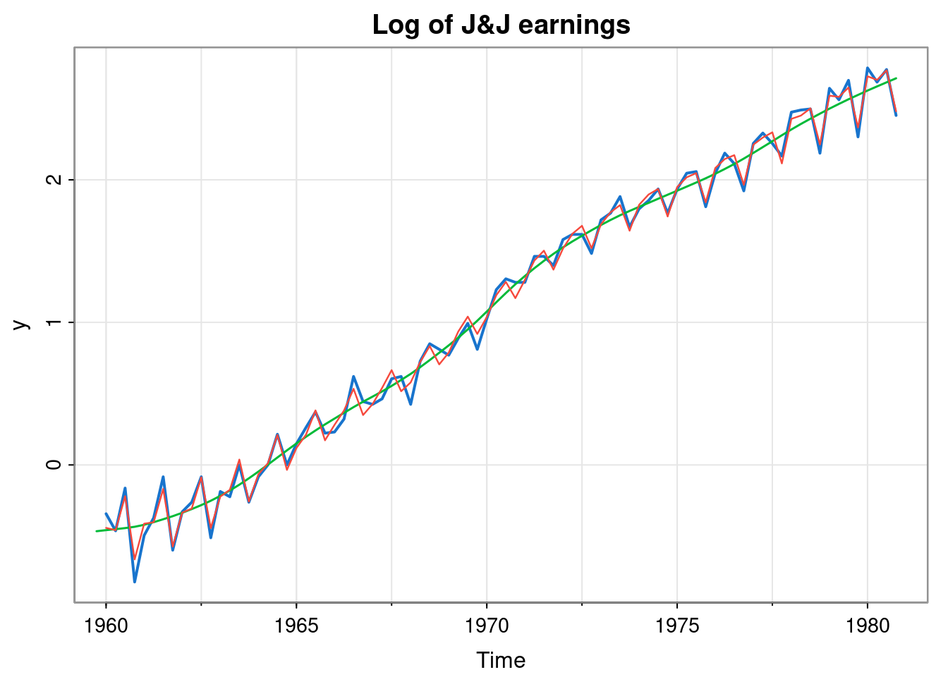
Once we are happy that the model is a good fit to the data, we can use it for forecasting.
fit = dlmFilter(y, mod)
fore = dlmForecast(fit, 16) # forecast 16 time points
pred = ts(c(tail(y, 1), fore$f),
  start=end(y), frequency=frequency(y))
upper = ts(c(tail(y, 1), fore$f + 2*sqrt(unlist(fore$Q))),
  start=end(y), frequency=frequency(y))
lower = ts(c(tail(y, 1), fore$f - 2*sqrt(unlist(fore$Q))),
  start=end(y), frequency=frequency(y))
all = ts(c(y, upper[-1]), start=start(y),
  frequency = frequency(y))
tsplot(all, ylab="log(earnings)",
  main="Forecasts with 2SD intervals")
lines(y, col=4, lwd=1.5)
lines(pred, col=2, lwd=2)
lines(upper, col=2)
lines(lower, col=2)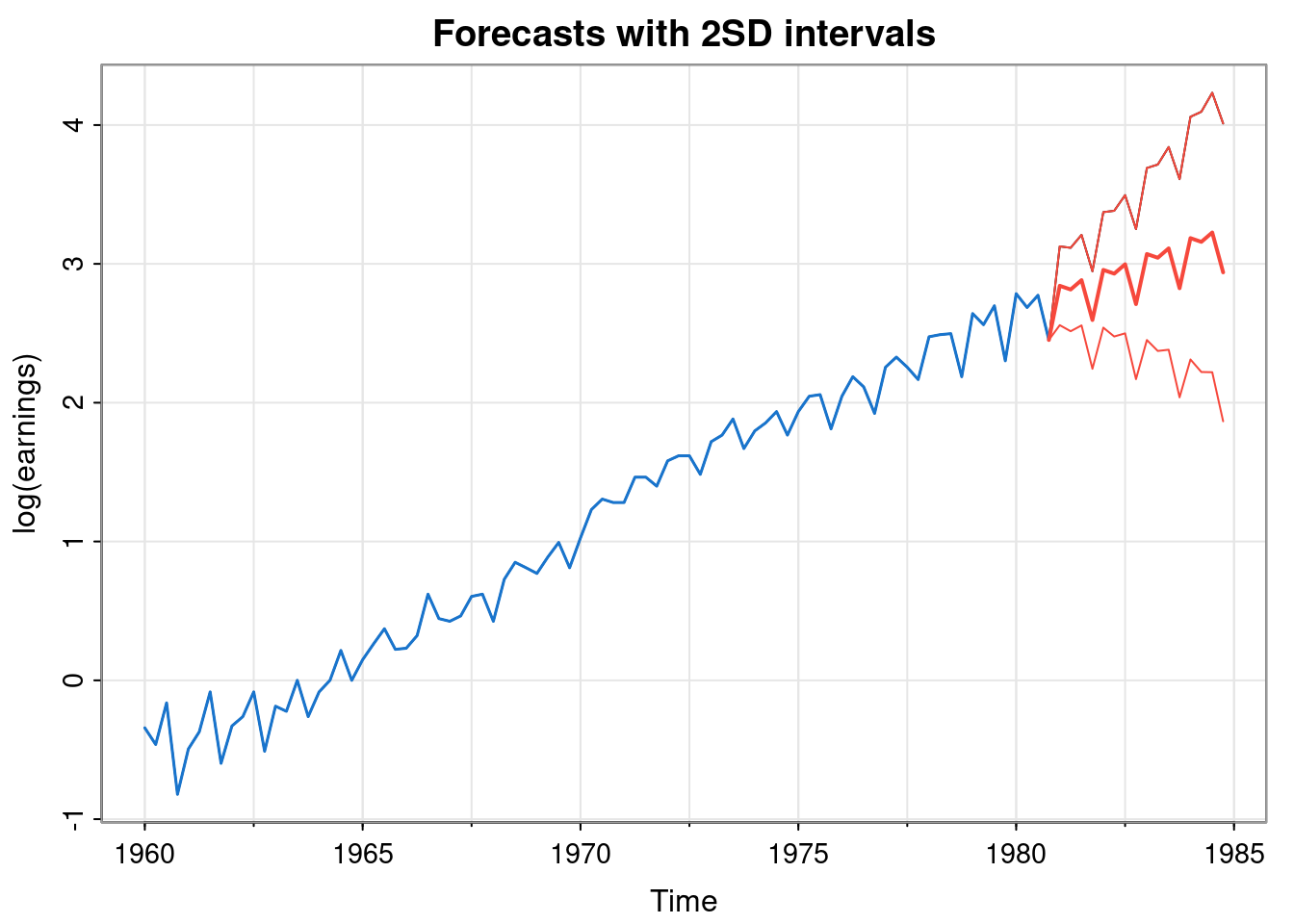
8.4.1 Example: monthly births
For an additional example, we will look at monthly live birth data for the US.
y = birth
tsplot(y, col=4, lwd=1.5, main="Monthly births")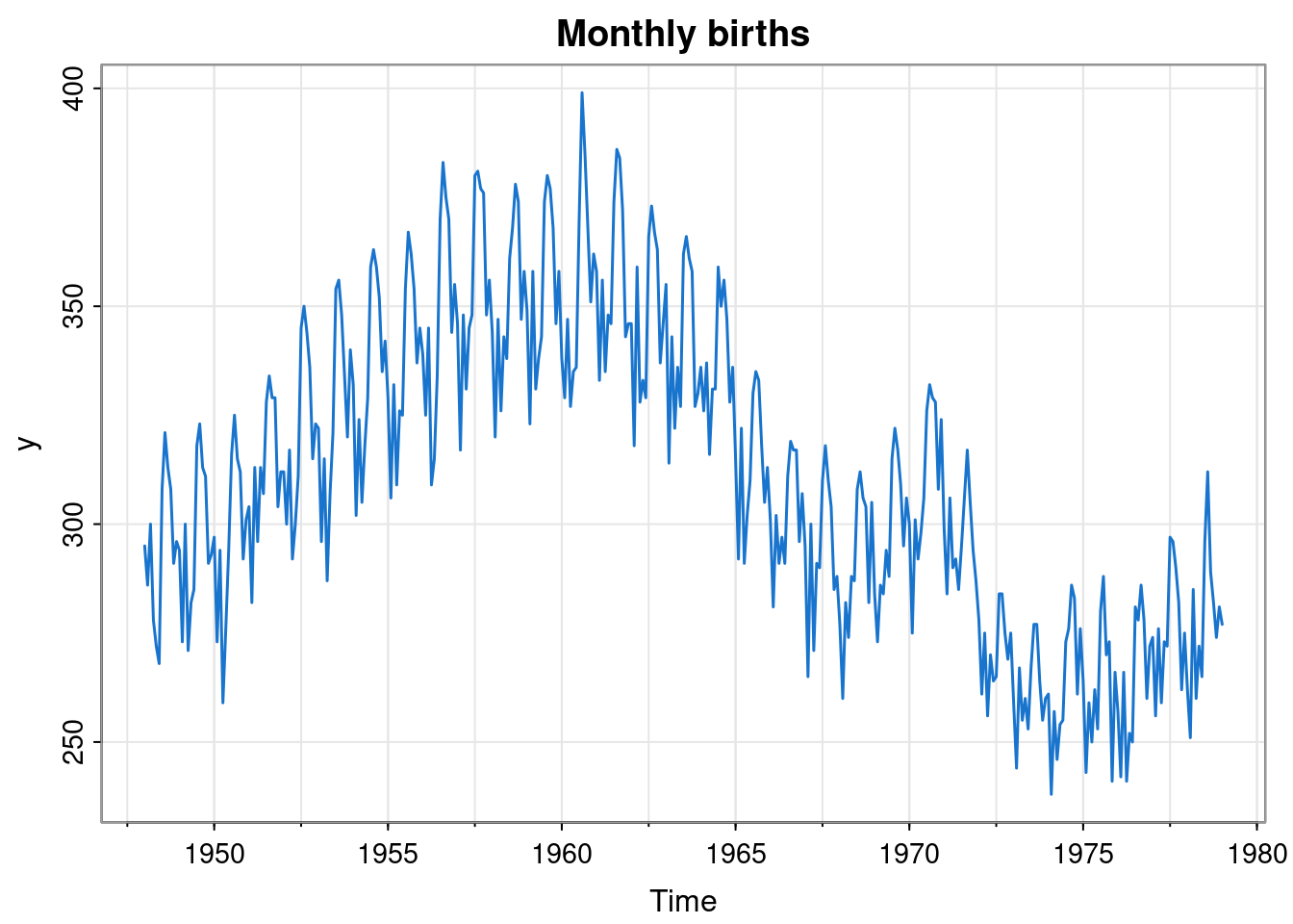
This seems to have a random walk nature, but with a strong seasonal component. We will assume that we do not want to use a full seasonal model, and instead use a seasonal model based on Fourier components with two harmonics. We may be unsure as to what variances to assume, and so want to estimate those using maximum likelihood. We could fit this using the dlm package as follows.
buildMod = function(lpar)
  dlmModPoly(1, dV=exp(lpar[1]), dW=exp(lpar[2])) +
    dlmModTrig(12, 2, dV=0, dW=rep(exp(lpar[3]), 4))
opt = dlmMLE(y, parm=log(c(100, 1, 1)),
        build=buildMod)
opt
$par
[1] 4.482990 1.925763 -3.228793
$value
[1] 1116.91
$counts
function gradient
14 14
$convergence
[1] 0
$message
[1] "CONVERGENCE: REL_REDUCTION_OF_F <= FACTR*EPSMCH"mod = buildMod(opt$par)
ss = dlmSmooth(y, mod)
so = ss$s[-1,] %*% t(mod$FF) # smoothed observations
so = ts(so, start(y), frequency = frequency(y))
tsplot(y, col=4, lwd=1.5, main="Monthly births")
lines(ss$s[,1], col=3, lwd=1.5)
lines(so, col=2, lwd=1.2)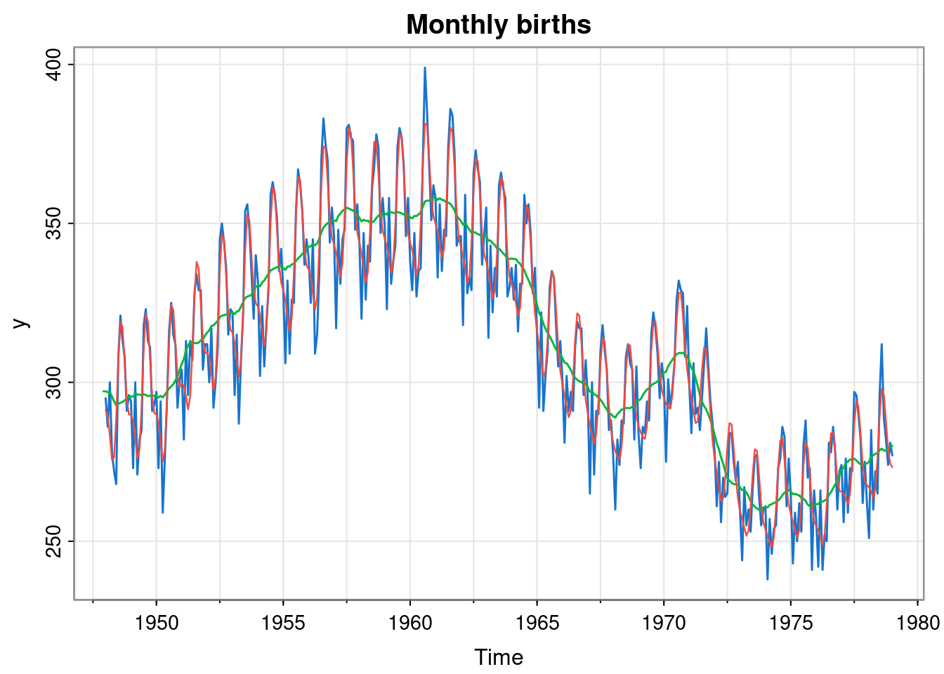
The optimised parameters seem to correspond to a good fit to the data.
8.5 ARMA models in state space form
We have seen in previous chapters how ARMA models define a useful class of discrete time Gaussian processes that can effectively capture the kinds of auto-correlation structure that we often see in time series. They can be useful building blocks in DLM models. To use them in this context, we need to know how to represent them in state space form.
8.5.1 AR models
In fact, we have already seen a popular way to represent an AR\((p)\) model as a VAR(1), and this is exactly what we need for state space modelling. So, to build a DLM representing noisy observation of a hidden AR\((p)\) model we specify \(\mathsf{F}=(1,0,\ldots,0)\), \[ \mathsf{G} = \begin{pmatrix} \phi_1&\cdots&\phi_{p-1}&\phi_p\\ 1&\cdots&0&0\\ \vdots&\ddots&\ddots&\vdots\\ 0&\cdots&1&0 \end{pmatrix}, \] \(\mathsf{W}=\operatorname{diag}(\sigma^2,0,\ldots,0)\), \(\mathsf{V}=(v)\). As a reminder of why this works, we see that if we define \(\mathbf{X}_t = (X_t,X_{t-1},\ldots,X_{t-p})^\top\), where \(X_t\) is our AR\((p)\) process, then \[ \mathsf{G} \mathbf{X}_{t-1} + \begin{pmatrix}\varepsilon_t\\0\\\vdots\\0\end{pmatrix} = \mathbf{X}_t, \] and so the VAR(1) update preserves the stationary distribution of our AR\((p)\) model. However, this VAR(1) representation of an AR\((p)\) model is by no means unique. In fact, it turns out that replacing the above \(\mathsf{G}\) with \(\mathsf{G}^\top\) gives a VAR(1) model which also has the required AR\((p)\) model as the marginal distribution of the first component. This is not so intuitive, but generalises more easily to the ARMA case, so it is worth understanding. For this case we instead define the state vector to be \[ \mathbf{X}^\star_t = \begin{pmatrix} X_t\\ \phi_2X_{t-1}+\phi_3X_{t-2}+\ldots+\phi_pX_{t-p+1}\\ \vdots\\ \phi_{p-1}X_{t-1}+\phi_pX_{t-2}\\ \phi_pX_{t-1} \end{pmatrix}, \] where \(X_t\) is our AR\((p)\) process of interest, and note that only the first component of this state vector has the distribution we require. But with this definition we have \[ \mathsf{G}^\top\mathbf{X}^\star_{t-1} + \begin{pmatrix}\varepsilon_t\\0\\\vdots\\0\end{pmatrix} = \mathbf{X}^\star_t, \] and so this VAR(1) update preserves the distribution of this state vector. Consequently, the first component of the VAR(1) model defined this way will be marginally our AR\((p)\) model of interest. This representation is commonly encountered in practice, since the same approach works for ARMA models, where it is necessary to carry information about “old” errors in the state vector.
8.5.2 ARMA models
Representing an arbitrary ARMA model as a VAR(1) is also possible, and again the representation is not unique. However, the second approach that we used for AR\((p)\) models can be adapted very easily to the ARMA case. Consider first an ARMA\((p, p-1)\) model, so that we have one fewer MA coefficients than AR coefficients. Using the \(p\times p\) auto-regressive matrix \[ \mathsf{G} = \begin{pmatrix} \phi_1 & 1 & \cdots & 0 \\ \vdots & \vdots & \ddots & \vdots \\ \phi_{p-1} & 0 &\ddots & 1 \\ \phi_p & 0 & \cdots & 0 \end{pmatrix}, \] together with the error vector \[ \pmb{\varepsilon}_t = \begin{pmatrix}1\\\theta_1\\\vdots\\\theta_{p-1}\end{pmatrix}\varepsilon_t, \] leads to a hidden state vector with first component marginally the ARMA\((p,p-1)\) process of interest. Note that the error covariance matrix is \[ \mathsf{W} = \begin{pmatrix}1\\\theta_1\\\vdots\\\theta_{p-1}\end{pmatrix} \begin{pmatrix}1\\\theta_1\\\vdots\\\theta_{p-1}\end{pmatrix}^\top\sigma^2. \] To understand why this works, define our state vector to be \[ \mathbf{X}_t = \begin{pmatrix} X_t\\ \phi_2X_{t-1}+\phi_3X_{t-2}+\ldots+\phi_pX_{t-p+1}+\theta_1\varepsilon_{t}+\cdots+\theta_{p-1}\varepsilon_{t-p+2}\\ \vdots\\ \phi_{p-1}X_{t-1}+\phi_pX_{t-2}+\theta_{p-2}\varepsilon_t+\theta_{p-1}\varepsilon_{t-1}\\ \phi_pX_{t-1}+\theta_{p-1}\varepsilon_t \end{pmatrix}. \] We can then directly verify that \[ \mathsf{G}\mathbf{X}_{t-1} + \pmb{\varepsilon}_t = \mathbf{X}_t, \] and so this VAR(1) update preserves the distribution of our state vector. Consequently, the first component is marginally ARMA, and so using \(\mathsf{F}=(1,0,\cdots,0)\) will pick out this component for incorporation into the model of observation process.
We have considered the case of ARMA\((p,p-1)\), but note that any ARMA\((p,q)\) model can be represented as an ARMA\((p^\star,p^\star-1)\) model by choosing \(p^\star=\max\{p,q+1\}\) and padding coefficient vectors with zeros as required. This is exactly the approach used by the function dlm::dlmModARMA.
8.5.3 Example: SOI
Let us return to the SOI example we looked at at the end of Chapter 7. We can model this using a locally constant model, but also with a seasonal effect. Further, we can investigate any residual correlation structure by including an AR(2) component. We can fit this as follows.
y = soi
buildMod = function(param)
  dlmModPoly(1, dV=exp(param[1]), dW=exp(param[2])) +
    dlmModARMA(ar=c(param[3], param[4]),
     sigma2=exp(param[5]), dV=0) +
    dlmModTrig(12, 2, dV=0, dW=rep(exp(param[6]), 4))
opt = dlmMLE(y, parm=c(log(0.1^2), log(0.01^2),
  0.2, 0.1, log(0.1^2), log(0.01^2)), build=buildMod)
opt
$par
[1] -3.100868e+00 -9.242014e+00 8.792923e-01 -7.119263e-06 -4.572246e+00
[6] -1.010190e+01
$value
[1] -310.9818
$counts
function gradient
51 51
$convergence
[1] 0
$message
[1] "CONVERGENCE: REL_REDUCTION_OF_F <= FACTR*EPSMCH"mod = buildMod(opt$par)
ss = dlmSmooth(y, mod)
so = ss$s[-1,] %*% t(mod$FF) # smoothed observations
so = ts(so, start(y), freq=frequency(y))
tsplot(y, col=4, lwd=1.5, main="SOI")
lines(ss$s[,1], col=3, lwd=1.5)
lines(so, col=2)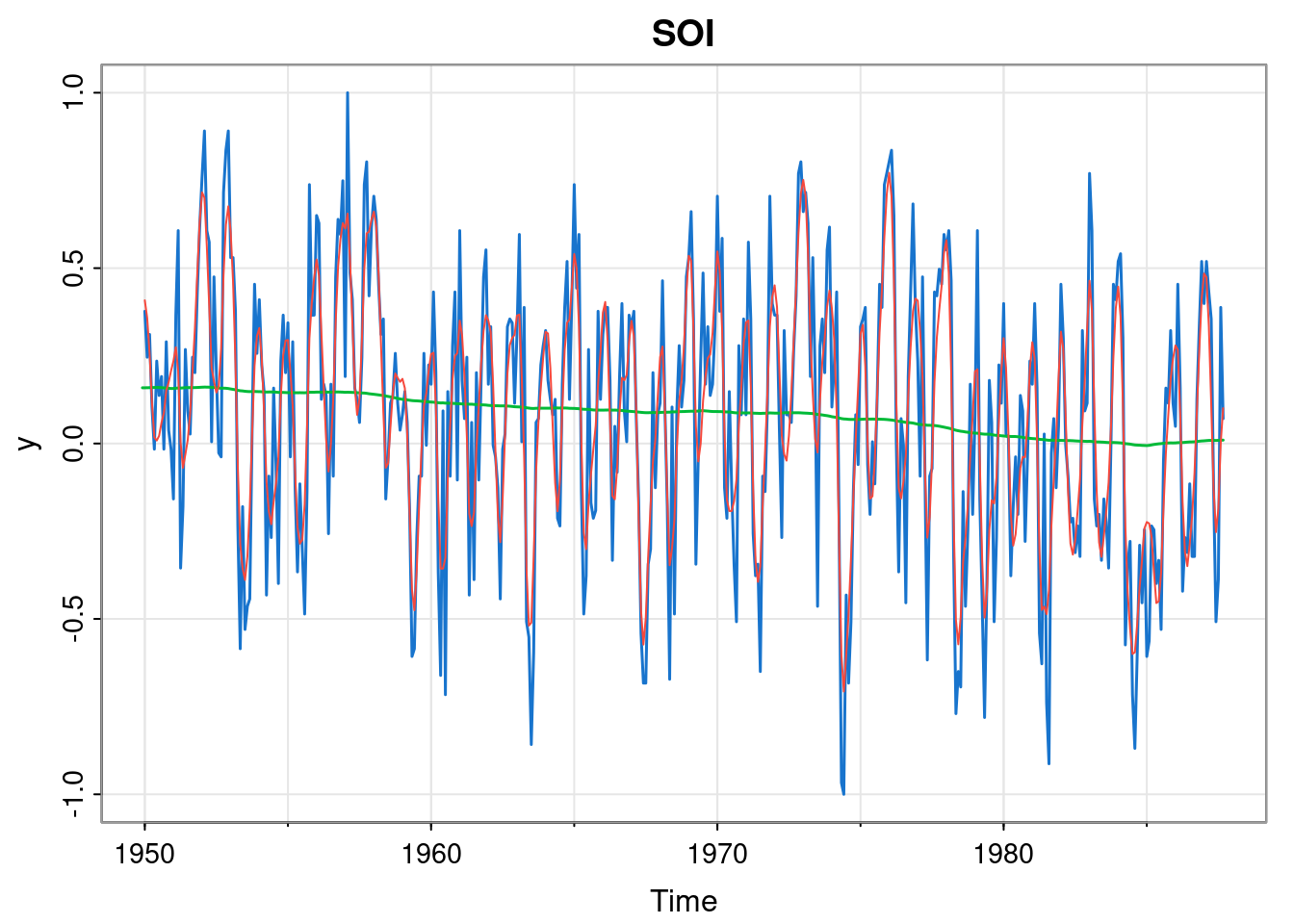
This looks to be a good fit, suggesting a gradual slow decreasing trend, but inspection of the optimised parameters (in particular param[5], the log of \(\sigma^2\) in the ARMA component), suggests that the AR(2) component is not necessary.
8.6 Multivariate models
The DLM formalism introduced in Chapter 7 covers multivariate observations of dimension \(m\). Each of the \(m\) rows of \(\mathsf{F}\) determines how the state vector is transformed into a component of the observation vector. However, the process of building an appropriate model for multivariate data is considerably more challenging than for univariate time series. Here we will give a brief introduction to some of the most important concepts. We will then revisit the topic later in the context of spatio-temporal data, which can often be sensibly regarded as a multivariate time series with special (spatial) structure.
For our running example we will use part of the astsa::lap dataset. This contains weekly data on various pollutant levels, in addition to some mortality data. To keep things simple, we will just focus on three (correlated) pollution variables, co (Carbon monoxide), no2 (Nitrogen dioxide) and part (Particulate matter).
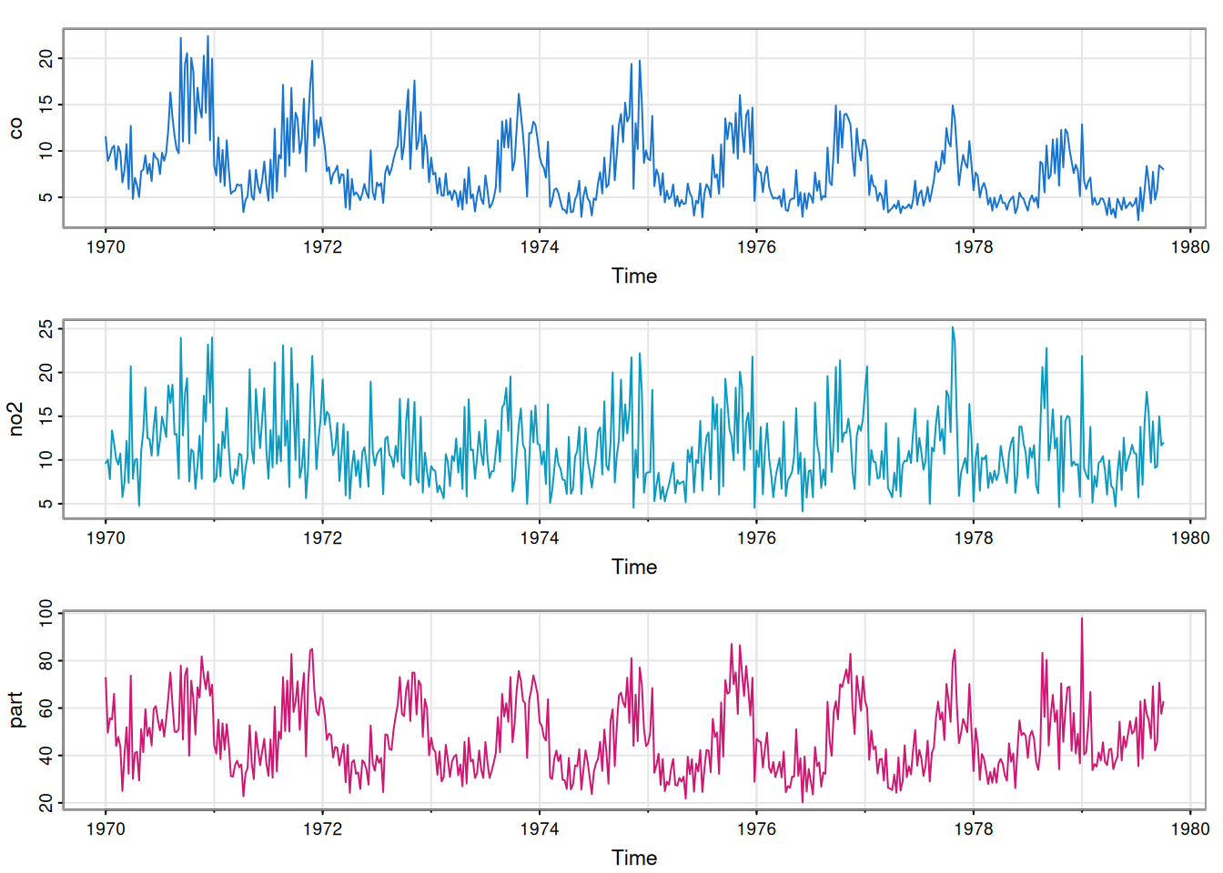
We see that each component is seasonal, with peaks occurring at similar times of the year. This will certainly lead to associate between the component series, as can be confirmed with a pairs plot.
pairs(pol, col=4, pch=19)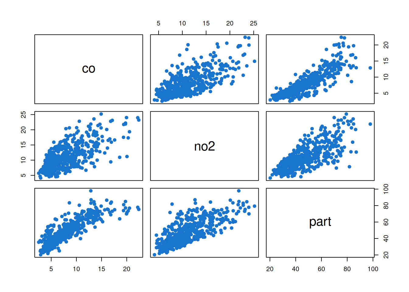
What is much less obvious at this stage is whether the association is entirely due to the seasonality, or whether there is residual correlation between the series even after accounting for other factors. We will need to carefully model the data in order to obtain a satisfactory understanding of this issue.
We will begin our modelling process by developing appropriate univariate models for each component, and then think about how to combine them into a multivariate model in an appropriate way. From a basic eye-balling of the data, it appears that each series can probably be reasonably well described by a locally constant model with a seasonal component that isn’t too complicated, so may be reasonably described with two Fourier components. However, the time series all look different, so each component will need to be parameterised separately. A basic model building function is given below.
buildMod = function(lpar) {
    par = exp(lpar)
    dlmModPoly(1, dV=par[1], dW=par[2]) +
        dlmModTrig(52, 2, dV=0, dW=rep(par[3], 4))
}
We can use this function to parameterise each component in turn. We will start with carbon monoxide.
[1] 4.4767675057 0.0135413012 0.0004923974p1Mod = buildMod(opt$par)
ss = dlmSmooth(pol[,1], p1Mod) # smoothed states
so = ss$s[-1,] %*% t(p1Mod$FF) # smoothed obs
so = ts(so, start(pol[,1]), freq=frequency(pol[,1]))
tsplot(pol[,1], col=4, main="CO")
lines(ss$s[,1], col=3, lwd=1.5) # current level
lines(so, col=2, lwd=1.5)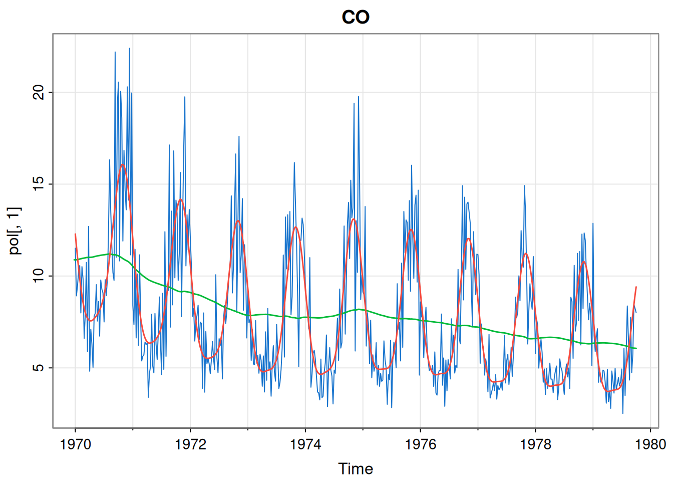
[1] 697.7364The dlmMLE function seems to have found a good fit for this component. We can do the same for nitrogen dioxide.
[1] 1.387212e+01 6.254836e-03 8.642782e-04p2Mod = buildMod(opt$par)
ss = dlmSmooth(pol[,2], p2Mod) # smoothed states
so = ss$s[-1,] %*% t(p2Mod$FF) # smoothed obs
so = ts(so, start(pol[,2]), freq=frequency(pol[,2]))
tsplot(pol[,2], col=5, main="NO2")
lines(ss$s[,1], col=3, lwd=1.5)
lines(so, col=2, lwd=1.5)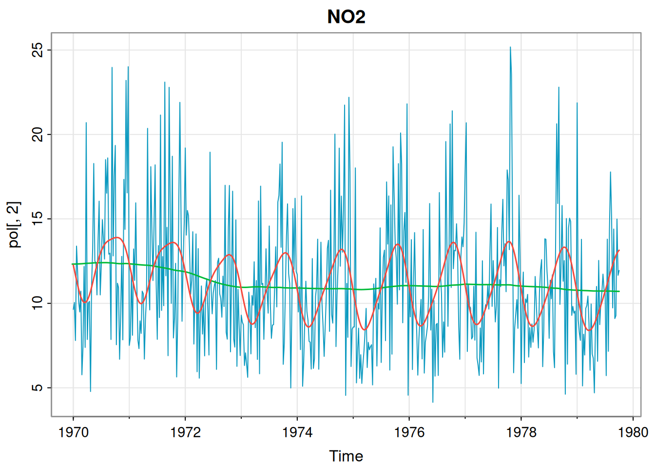
[1] 973.3261This fit also seems fine. Finally we repeat for particulate matter.
[1] 90.65737051 0.14812352 0.07025641p3Mod = buildMod(opt$par)
ss = dlmSmooth(pol[,3], p3Mod) # smoothed states
so = ss$s[-1,] %*% t(p3Mod$FF) # smoothed obs
so = ts(so, start(pol[,3]), freq=frequency(pol[,3]))
tsplot(pol[,3], col=6, main="Particulate")
lines(ss$s[,1], col=3, lwd=1.5)
lines(so, col=4, lwd=1.5)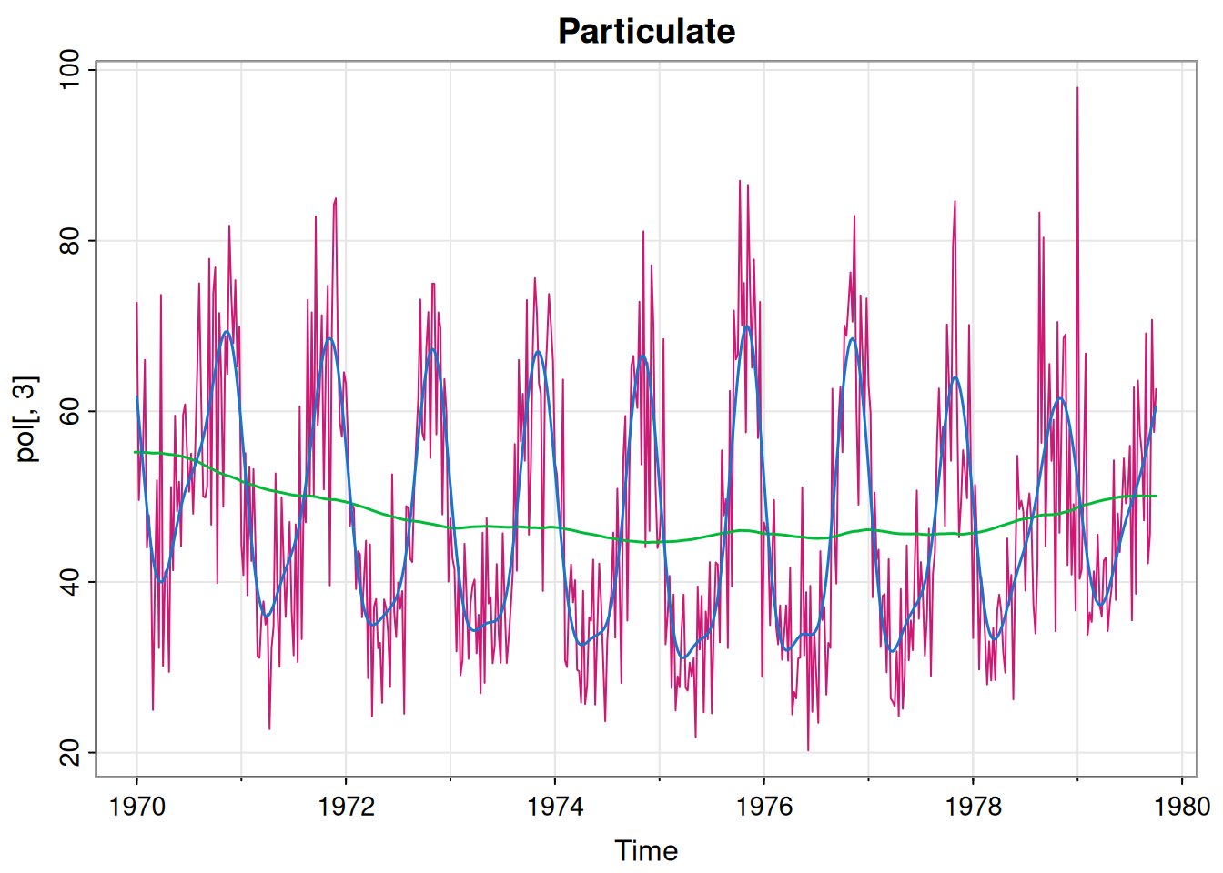
[1] 1460.519This also seems fine. So, we now have three perfectly reasonable univariate models. If we believe that all of the series are truly independent of one another then this is fine. However, if we think that there may be dependencies and correlations between the components that are not accounted for by fitting univariate models independently, then we need a proper multivariate DLM for the 3-dimensional observation vector.
8.6.1 Model concatenation
There is an obvious way to glue together independent DLMs to form a combined DLM that is entirely equivalent. The operation is quite similar to the model superposition operation considered in Section 8.4, but importantly different. Here we suppose that we have two models. Model \(i\) (for \(i=1,2\)) has state dimension \(p_i\), observation dimension \(m_i\) and is defined by \(\{\mathsf{G}_{it}, \mathsf{F}_{it}, \mathsf{W}_{it}, \mathsf{V}_{it}\}\). Their concatenation or outer sum is a model with state dimension \(p_1+p_2\) and observation dimension \(m_1+m_2\) defined by \[ \bigg\{ \text{blockdiag}\{\mathsf{G}_{1t},\mathsf{G}_{2t}\}, \text{blockdiag}\{\mathsf{F}_{1t},\mathsf{F}_{2t}\}, \text{blockdiag}\{\mathsf{W}_{1t},\mathsf{W}_{2t}\}, \text{blockdiag}\{\mathsf{V}_{1t},\mathsf{V}_{2t}\} \bigg\} \] Note that the component models are entirely independent of one another, so this model is entirely equivalent to the separate models (and hence not intrinsically better). Again, this operation can clearly be repeated to combine multiple models, and the operation is clearly associative.
This outer sum is implemented in the dlm package using the %+% operator.
     [,1] [,2] [,3] [,4] [,5] [,6] [,7] [,8] [,9] [,10] [,11] [,12] [,13] [,14]
[1,]    1    1    0    1    0    0    0    0    0     0     0     0     0     0
[2,]    0    0    0    0    0    1    1    0    1     0     0     0     0     0
[3,]    0    0    0    0    0    0    0    0    0     0     1     1     0     1
     [,15]
[1,]     0
[2,]     0
[3,] 0print(polMod$V) [,1] [,2] [,3]
[1,] 4.476768 0.00000 0.00000
[2,] 0.000000 13.87212 0.00000
[3,] 0.000000 0.00000 90.65737[1] 3131.581Computing the (negative) log-likelihood of the combined model gives us the sum of the log-likelihoods of the component models, as we would expect. As discussed, this independent component model is equivalent to the separate univariate models, so not yet any better. However, this is a good “straw man” multivariate model that we can use as a starting point for building a better, more fundamentally multivariate model.
8.6.2 Multivariate dependence
Now that we have a reasonable model based on an assumption of independence between the components, we can investigate whether there appear to be any dependencies between the components that are not just indirect associations due to similar patterns of seasonality. We begin by looking at the “residuals” for the base model. We can form residuals by subtracting the fitted smoothed observations from the actual observations.
ss = dlmSmooth(pol, polMod)
so = ss$s[-1,] %*% t(polMod$FF)
so = ts(so, start(pol), freq=frequency(pol))
resid = pol - so
tsplot(resid, col=4:6)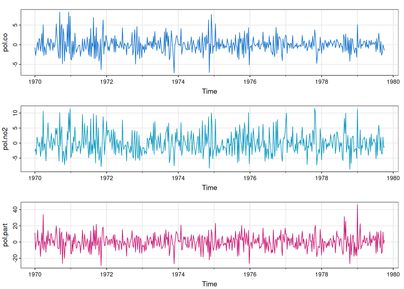
We see that each component residual time series looks fairly random, suggesting that our univariate models are all reasonable fits. But are there any cross-correlations between the residual components?
pairs(resid, col=4, pch=19, cex=0.5)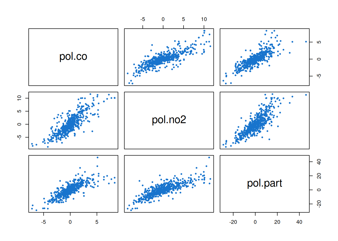
Clearly there are. This is strongly suggestive that our base model could be improved by building some kind of dependence between the components. There are many ways that this could be done. The simplest approach may be to allow some correlation in the \(\mathsf{V}\) or \(\mathsf{W}\) matrices. But in some cases in can also make sense to couple the components by introducing additional non-zero off-diagonal elements into the \(\mathsf{G}\) matrix. Exploring these things in detail is beyond the scope of this course. For now we will just see how allowing correlations in the \(\mathsf{V}\) matrix can greatly improve the model fit. Comparing the covariance matrix of the residuals with the current fitted \(\mathsf{V}\) matrix
            pol.co   pol.no2 pol.part
pol.co    4.288101  6.225905 15.40535
pol.no2   6.225905 13.535552 27.90618
pol.part 15.405352 27.906175 85.62305print(polMod$V) [,1] [,2] [,3]
[1,] 4.476768 0.00000 0.00000
[2,] 0.000000 13.87212 0.00000
[3,] 0.000000 0.00000 90.65737shows that while the diagonal is similar, the residuals have strong cross-correlations that are currently absent from our model. We could directly optimise a model with a parameterised covariance matrix, but this requires a little care due to the positive-definiteness constraint. For illustrative purposes, we can just replace the existing \(\mathsf{V}\) matrix with the empirical covariance matrix of the residuals.
We see that this leads to a massive improvement in the model likelihood (the negative log-likelihood is much smaller). So this is now a much better fitting model, and should therefore lead to improved smoothing and forecast distributions. Of course, other model refinements could also help, but we leave investigation of this to the interested reader.
As previously discussed, multivariate time series modelling is a big topic, and good models usually rely on very specific features of the multivariate data under consideration. Spatio-temporal data is a good example of multivariate time series with special structure, and we will see how this can be exploited at the end of the course, once we know a bit about spatial modelling.